Benchmark Applications

Overview of Benchmark Applications

DynaSOAr was designed for SMMO applicatons and we claim that many applications can be written in SMMO style. In the following, we give an overview of the SMMO applications that we implemented with DynaSOAr. These applications are located in the example directory and we recommend following the source code when reading through this section.

We provide a build script for every application. There are a few command line options that most scripts understand:

• -d: Run in debug mode. This prints additional information about the state of the allocator and the layout of objects within blocks. Moreover, if DynaSOAr runs out of memory, the application crashes instead of going into an infinite loop.
• -r: Produces a graphical rendering. Requires the libsdl2 library.
• -a ALLOC: Use a custom allocator, where ALLOC can be one of dynasoar, bitmap, cuda, mallocmc, halloc.
• -m NUM_OBJ: Specifies the heap size of dynasoar/bitmap in terms of the maximum number of objects of the smallest type. Also affects the size of parallel do-all data structures when using other allocators.
• -s BYTES: Specifies the heap size of a custom allocator (not dynasoar or bitmap) in bytes.
• -x SIZE: Specifies the problem size. This is application-specific. This option is not available for gol, as that benchmark loads an initial state of fixed size from an external file.

If no heap size or problem size is specified, the benchmark falls back to the default size. That is the same size that we used for benchmarking in our paper. The default size may require a large amount of memory (around 8 GiB for some benchmarks).

To run the applications (using DynaSOAr) on a smaller GPU (at least 1 GiB of memory) and with graphical output, use the following shell snippets for compilation. (Tested with a GeForce 940MX GPU.)

nbody: Basic Particle System

$ build_scripts/build_nbody.sh -r -m 262144 -x 50
$ bin/nbody_dynasoar

This a simple 2D n-body simulation. Every body is an object and has fields for position, velocity, mass, etc. This is one of the simplest DynaSOAr examples. It illustrates its API and DSL, but there is no dynamic (de)allocation of objects after initialization.

Every iteration simulates a fixed time step and consists of two parallel do-all operations.

1. Body::compute_force(): Computes the force that acts on each body. The implementation of compute_force contains a (sequential) do-all operation (device_do) to compute the force between all pairs of bodies.
2. Body::update(): Computes the new velocity and position of each body. Bodies bounce off the walls before they go out of range.

collision: Particle System with Collisions

$ build_scripts/build_collision.sh -r -m 262144 -x 100
$ bin/collision_dynasoar

This is a modification of nbody, in which two bodies are merged if they are getting too close. This benchmark is interesting because it shows dynamic deallocation and a wider range of OOP features (e.g., member access operator -> for method calls).

Every iteration consists of 6 parallel do-all operations.

1. Body::compute_force(): Same as before.
2. Body::update(): Same as before.
3. Body::initialize_merge(): Resets fields that are used to implement merging behavior.
4. Body::prepare_merge(): Checks every pair of bodies to see if they are close enough for merging (using a device_do). If so, sets the merge_target of the giving object and has_incoming_merge of the receiving object.
5. Body::update_merge(): Physically merges a body into another one if merge_target is set and the receiving object does not have a merge target itself.
6. Body::delete_merged(): Deletes giving objects.

Note that this algorithm is not deterministic. The runtime scheduling of threads may determine which bodies get merged if there are multiple bodies in range.

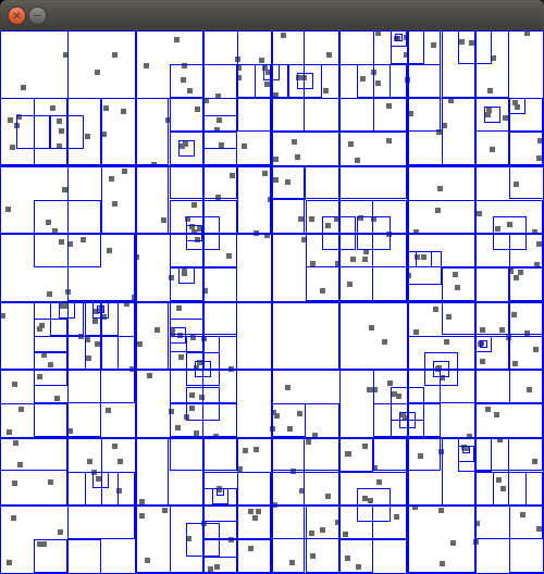
barnes-hut: Dynamic Tree Construction Benchmark

$ build_scripts/build_barnes_hut.sh -m 262144 -x 300 -r
$ bin/barnes_hut_dynasoar

This benchmark is another particle system. However, the focus of this application is on constructing a quad tree and keeping it up to date. This benchmark is interesting because it shows that DynaSOAr is suitable for dynamic tree structures.

There are three classes in this application. An abstract NodeBase class and two subclasses BodyNode and TreeNode. Every TreeNode has four children which may be nullptr or another NodeBase pointer. Moreover, every TreeNode stores the mass of all of its children and the position of the gravitational center. Barnes-Hut is faster than a normal n-body simulation, because, when computing the forces, TreeNodes can be utilized for reducing the number of object pairs: If a body is far enough away from a TreeNode, it is not necessary to traverse its children.

This application is quite complex and requires atomicCAS in application code. Every iteration consists of 4 steps.

1. Generate tree summaries (BFS).
2. Perform n-body simulation time step. Similar to n-body, but does a top-down traversal of the quad tree instead of iterating over all other body objects.
3. Update the tree.
4. Remove empty tree nodes (BFS).

Generating Tree Summaries

This step updates the mass and center of gravity of every tree node. It is implemented with a bottom-up BFS (parallel frontier-based BFS algorithm). Step 2 and 3 are repeated until the root of the tree was updated.

1. TreeNode::initialize_frontier(): If the tree node is a leaf, make it part of the frontier.
2. TreeNode::bfs_step(): Compute mass and center of gravity based on the child nodes. Remove the node from the frontier.
3. TreeNode::update_frontier(): If the node was not processed yet but all of its children were, make it part of the frontier.

Updating the Tree

This step consists of two parallel do-all operations.

1. BodyNode::clear_node(): If this body is out of the bounds of its parent, remove it from its parent.
2. BodyNode::add_to_tree(): This is the most difficult part of the implementation. If a body has no parent, insert it into the tree. This is done with a top-down traversal of the quad tree and atomic node replacements.

Removing Empty Tree Nodes

This step removes tree nodes that have no children. It is implemented with a bottom-up BFS. Steps 2 and 3 are repeated until the root of the tree was visited.

1. TreeNode::initialize_frontier(): If the tree node is a leaf, make it part of the frontier.
2. TreeNode::collapse_tree(): If the node has no children, remove it from its parent and deallocate it.
3. TreeNode::update_frontier(): If the node was not processed yet but all of its children were, make it part of the frontier.

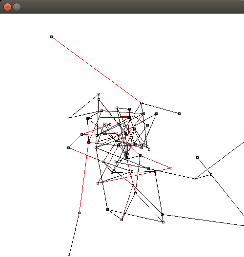
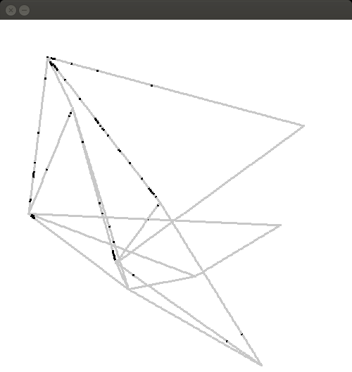
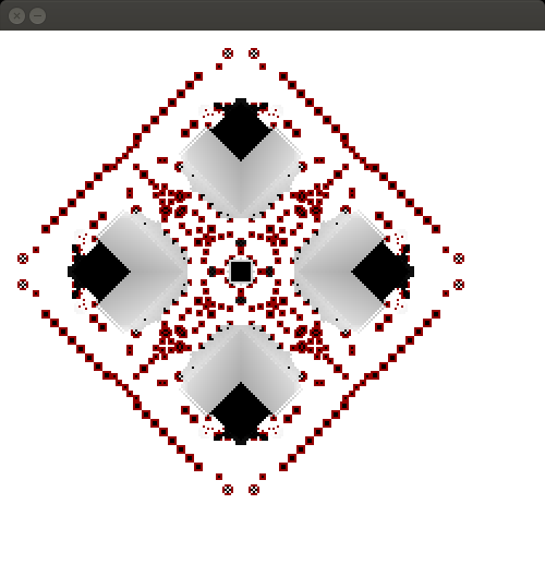
structure: Finite Element Method (FEM)

$ build_scripts/build_structure.sh -x 80 -r -m 262144
$ bin/structure_dynasoar

This is a simulation of a fracture in a material using a finite element method. Interestingly, a modified version of this algorithm can also be used for graph layouting.

The simulation consists of a number of elements/nodes (class Node). Nodes have a position, velocity and mass. Nodes are connected with each other through springs (class Spring). Springs pull the nodes closer to each other (Hooke's law), but not closer than their original distance. If the force of a spring exceeds a certain threshold, it breaks. Disconnected nodes (and springs) are detected with a BFS and removed from the simulation. There are three kinds of nodes: Ordinary nodes (class Node), nodes that do not move (anchor nodes, class AnchorNode) and nodes that move with a fixed velocity into a certain direction (pull nodes, class AnchorPullNode).

Every iteration in this simulation consists of a number of parallel do-all operations.

1. AnchorPullNode::pull(): Anchor pull nodes are moved into a certain direction.
2. Compute step (repeat 40 times).
3. Remove disconnected nodes and springs (BFS).

Compute Step

A compute step consists of 2 parallel do-all operations (compute()):

1. Spring::compute_force(): Every spring computes its force according to Hooke's law. If the force exceeds a threshold, it removes itself from both node endpoints and then deletes itself.
2. Node::move(): Every node sums up the forces of all connected springs, calculates a new velocity and updates its position.

Removing Disconnected Nodes

This step consists of 4 parallel do-all operations (bfs_and_delete()). Step 2 is repeated until the entire graph was visited.

1. NodeBase::initialize_bfs(): We start BFS from anchor nodes, so the BFS distances of these nodes are set to 0. The distances of the other nodes are set to infinite.
2. NodeBase::bfs_visit(distance): distance increases by 1 with every iteration. Nodes with that distance are part of the frontier and are being processed in the current iteration.
3. NodeBase::bfs_set_delete_flags(): Springs connected to unvisited nodes are marked for deletion.
4. Spring::bfs_delete(): Springs that are marked for deletion are deleting themselves. Once a node has no springs anymore, it is also deleted.

This simulation generates a random graph and then runs 500 iterations.

sugarscape: Simulation of Population Dynamics

$ build_scripts/build_sugarscape.sh -x 100 -r -m 262144
$ bin/sugarscape_dynasoar

Sugarscape is an agent-based social simulation. There are different variants that can simulate different aspects of a population. To keep the benchmark simple, we are focusing on the movement of agents, ageing and mating.

The simulation consists of a 2D grid of cells. Every cell can store a certain amount of "sugar", which is a resource that agents need to survive. Every cell has a certain sugar grow rate. There are male and female agents, which can move to neighboring cells. Agents consume sugar and can mate when they are close enough, spawning a new agent. Every agent has properties such as a certain range of vision, metabolism rate, etc. These properties are passed down to offspring.

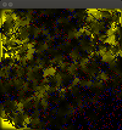
Every iteration in this simulation consists of 12 do-all operations. We do not describe every operation in detail here, but there are operations for growing sugar, diffusing sugar to neighboring cells, ageing and consuming sugar, deciding onto which cell to move (similar logic to wa-tor, see below) and mating.

traffic: Nagel-Schreckenberg Traffic Flow Simulation

$ build_scripts/build_traffic.sh -r -x 10 -m 16384
$ bin/traffic_dynasoar

This is an agent-based traffic flow simulation that implements the Nagel-Schreckenberg model. In this model, streets are divided into cells (class Cell). Every cell can hold at most one car (class Car). Every car has a velocity in "number of cells per iteration".

Every iteration in this simulation consists of 3 parallel do-all operations. This simulation also models traffic lights, but they are currently not implemented with DynaSOAr yet.

1. ProducerCell::create_car(): Cells that are classified as sources, produce a new car with a certain probability if the cell is empty.
2. Car::step_prepare_path(): First, the velocity of the car is increased by 1. Then, the car determines the next v cells where v is the velocity of the car. If one of these cells is currently occupied, the velocity is reduced, such that no occupied cell is entered (to avoid car collisions).
3. Car::step_move(): Every car moves to a cell of distance v, as computed by the previous step.

This simulation generates a random street network with -x intersections. We also experimented with loading real OSM city maps, but we would like to keep this benchmark as simple as possible.

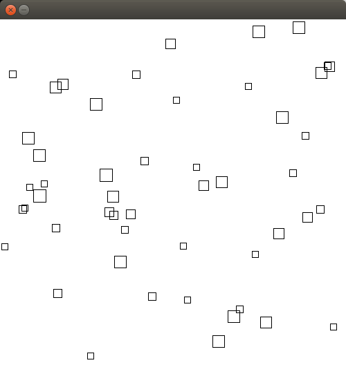
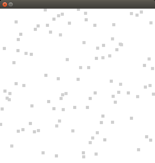
wa-tor: Fish-and-Sharks Simulation

$ build_scripts/build_wa_tor.sh -r -x 500 -y 500 -m 262144
$ bin/wator_dynasoar_no_cell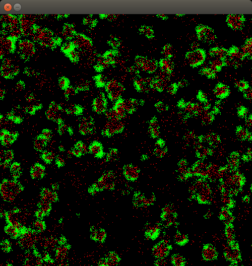

This is an agent-based predator-prey simulation. The green dots represent fish (class Fish) and the red dots represent sharks (class Shark). Both are moving on a 2D grid of cells (class Cell).

Every iteration in this simulation consists of 8 parallel do-all operations.

1. Cell::prepare(): There is a boolean flag neighbor_request for every neighbor of a cell. These flags are set to false.
2. Fish::prepare(): Every fish scans its neighboring cells. It selects a random free cell and sets the corresponding neighbor_request flag on the neighboring cell to true.
3. Cell::decide(): Every cells checks its neighbor_request flags to see which agents from neighboring cells want to enter this cell. It selects one of those cells at random.
4. Fish::update(): If a fish was selected, it moves onto the target cell and may create a new fish at its old location. Otherwise, it stays where it is.

There are 4 more do-all operations for sharks, which are implemented similarly.

gol: Game of Life

$ tar xvfz example/game-of-life/dataset/turing_machines.tar.gz -C example/game-of-life/dataset
$ build_scripts/build_gol.sh -r -d -m 262144
$ bin/gol_dynasoar_no_cell example/game-of-life/dataset/tm.pgm

This is an implementation of Game of Life. In most GOL implementations, every cell is mapped to a GPU thread. However, in this simulation, only alive cells and cells that may become alive soon are processed by GPU threads. There are 3 classes in this application: Cell, Agent and two subclasses of Agent; Alive and Candidate. The latter one is used for cells that are not alive yet but may become alive in the next iteration; i.e., cells with at least one alive neighboring cell.

Every iterations consists of 4 parallel do-all operations.

1. Candidate::prepare(): Determines if the underlying cell should become alive.
2. Alive::prepare(): Determines if the underlying cell should die.
3. Candidate::update(): Depending on the precomputed action of step 1, this object replaces itself with an Alive object, deletes itself or does nothing.
4. Alive::update(): Depending on the precomputed action of step 2, this object may delete itself. Moreover, if this object was just created in step 3, it creates Candidate objects on its surrounding cells.

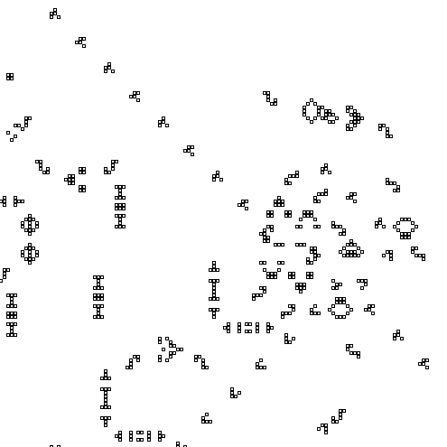
We tested this application with 2 datasets: A turing machine and a universial turning machine. The datasets were taken from Paul Rendell's website and are located in the dataset directory. Datasets must be stored in the PGM image format.

generation: Generational Cellular Automaton

$ build_scripts/build_generation.sh -m 8388608 -x 250 -r
$ bin/generation_dynasoar

This is an extension of gol. Alive cells have a state and block the cell for a certain period of time. The rule is based on Burst: 0235678/3468/255.

linux-scalability: Allocate/Deallocate Benchmark

$ build_scripts/build_linux_scalability.sh -x 8 -m 262144
$ bin/linux_scalability_dynasoar

We took this benchmark from the Linux Scalability project. It is not an SMMO application (no parallel do-all operations).

This application measures the raw (de)allocation time of an allocator. There are two CUDA kernels. The first kernel spawns 64 x 256 threads and every thread allocates a number of objects (64 bytes per object). The number of objects per thread can be specified with the -x command line parameter. The allocated memory is never accessed. The second kernel spawns the same number of threads and every thread deallocates the objects that it just allocated.