[2023-08-27] SFPN v0.1 is modified.
Single hyperspectral image (HSI) super-resolution (SR) methods using a auxiliary high-resolution (HR) RGB image have achieved great progress recently. However, most existing methods aggregate the information of RGB image and HSI early during input or shallow feature extraction, whose difference between two images has not been treated and discussed. Although a few methods combine both the image features in the middle layer of the network, they fail to make full use of the two inherent properties, i.e., rich spectra of HSI and HR content of RGB image, to guide model representation learning. To address these issues, in this article, we propose a dual-stage learning approach for HSI SR to learn a general spatial–spectral prior and image-specific details, respectively. In the coarse stage, we fully take advantage of two adjacent bands and RGB image to build the model. During coarse SR, a symmetrical feature propagation approach is developed to learn the inherent content of each image over a relatively long range. The symmetrical structure encourages the two streams to better retain their particularity. Meanwhile, it can realize the information interaction by the adaptive local block aggregation (ALBA) module. To learn image-specific details, a back-projection refinement network is embedded in the structure, which further improves the performance in fine stage. The experiments on four benchmark datasets demonstrate that the proposed approach presents excellent performance over the existing methods.
The deep-learning-based approaches have exhibited superior performance in natural image SR task. Recent works address HSI SR by referring to the SR algorithms for natural image including unsupervised and supervised manner. Compared with the traditional methods, these studies require less prior knowledge or none. Benefiting from the strong representation ability of the convolutional neural network, the unsupervised fusion approaches have made remarkable progress. However, these methods exist in two issues. The one is that some methods require multiple iterations when tested which increase the execution time. The other is that this type of methods obtains poor performance for real LR HSI, compared with the supervised deep-learning-based methods. Therefore, we focus on constructing a model in a supervised manner in our article.

Fig. 1. Visual comparison in spatial reconstruction on two dataset. The first and second lines are the visual images of the 10th and 20th bands, respectively. One can observe that our method obtains more bluer in the enlarged area. In particular, the contents around the edges are very light in this area.
Although public HSI dataset contains a small number of training samples, the researchers augment these data to train the model in a supervised manner. In contrast, the supervised fusion methods obtain better performance. Nevertheless, there are still some obvious shortcomings. For instance, most existing methods simply input HSI and HR RGB image into the model through the stack or in parallel, and integrate them at the beginning or initial feature extraction. Actually, there exists obvious distinction in edge texture between RGB image and HSI. This unites the two images prematurely, so that the difference between them has not been treated and discussed. While a few methods combine both the features in the middle layer of the network, they do not make effective use of significant properties, i.e., rich spectral information of HSI and HR content of RGB image. Concretely, HSI exhibits a remarkable characteristic that the adjacent bands have similarity. These adjacent bands help complement each other. Besides, as seen in Fig. 1, RGB image has sharper detail content than some bands. Ideally, the combination of these two properties is more favorable for the exploration of HSI SR, which makes the super-resolved image get clear details. Therefore, how to distinguish the differences between them and effectively make use of their significant properties is still an urgent problem to be solved.
LR HSI exhibits low spatial resolution, and its spectral resolution is actually still high. The main purpose of HSI SR is to improve the spatial resolution, leading to both high spatial and spectral resolution. Therefore, we should focus more on spatial study when establishing models. Besides, different from the RGB image, HSI has dozens or even hundreds of bands. When the spatial resolution and batch size of both the images are the same, the HSI requires more memory footprint after the input model than the RGB image. Under limited hardware resources, this puts forward higher requirements for model construction with more layers. One natural way is to reduce the batch size, but the training time will be greatly increased, making the parameter correction more slowly. When the batch size is set too small, the gradient descent direction of the model is not accurate, and the training results are easy to produce large shocks. This makes it difficult for the model to converge. Hence, the crucial issue is how to strengthen the exploration of spatial information while reducing the memory footprint.
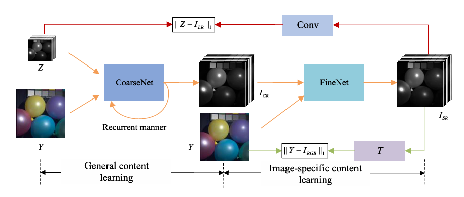
Considering this condition, we propose a symmetrical feature propagation network in the coarse stage, which is shown in Fig. 2. Specifically, inspired by the high correlation among neighboring bands, we use several bands and HR RGB image instead of inputting the whole HSI to achieve SR in the coarse stage. By doing so, it promotes the analysis of the spatial resolution of the current band. Besides, this approach alleviates the memory footprint only using several bands. To better apply adjacent spectral bands with high similarity, in our work, the current band and its two adjacent bands in the LR HSI are taken out separately and input into the network together with RGB image. It fully takes advantage of two inherent properties, namely, rich spectra of HSI and HR content of RGB image. Through the fusion in space between them, we obtain the current super-resolved band. All the bands are produced in the above way in a recurrent manner. During SR, the symmetrical multistep propagation mechanism is designed to make the model get better feature representation. It not only retains their particularity but also achieves the information interaction by means of separation-and-aggregation unit (SAU).
In the coarse stage, we only turn to the neighboring bands and ignore the relatively distant bands. Actually, these bands display distinct textures at diverse wavelengths (see Fig. 1). If they are handled effectively, it enables the model to yield clearer edges. In addition, CoarseNet only generates the general structure for LR HSI; however, it fails to describe image-specific details, such as LR HSI with unknown degeneration. Considering that there is a fixed transformation T between the initial result and RGB image, a back-projection refinement network is injected at the end of the structure to learn the image-specific details by cycle consistency loss, which can further refine the result. Note that all the initial bands and RGB image are simultaneously fed into the network in the fine stage.
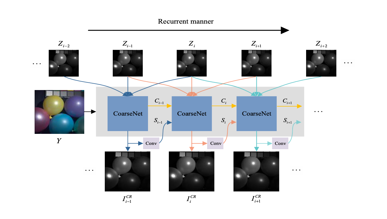
Fig. 2. Overview of the flowchart in the coarse stage. Only three bands (current band
Training Steps for Coarse Stage
Input: HR dataset
$\mathcal{D}$ and scale factor$s$
Output: Coarse model parameter$\theta_C$
Randomly initialize coarse model parameter$\theta$ ;
while not down do
Sample a batch of images {X} from dataset$\mathcal{D}$ ;
Generate {X, Z} by degradation, and obtain corresponding HR image Y using 1;
Set$i = 1$ ;
for$i≤L$ do
Evaluate$\mathcal{L}_C$ by 14 ;
Update$\theta$ according to$\mathcal{L}_C$ ;
$i \gets i+1$ ;
end
end
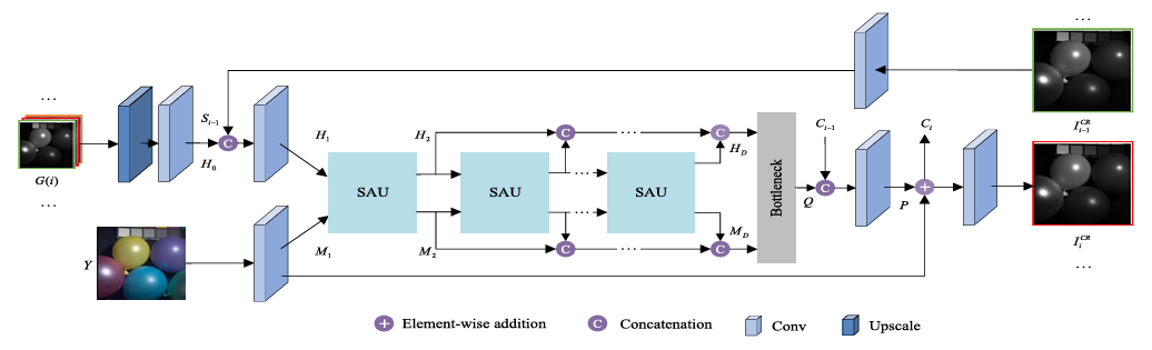
Fig. 3. Structure of the proposed CoarseNet.
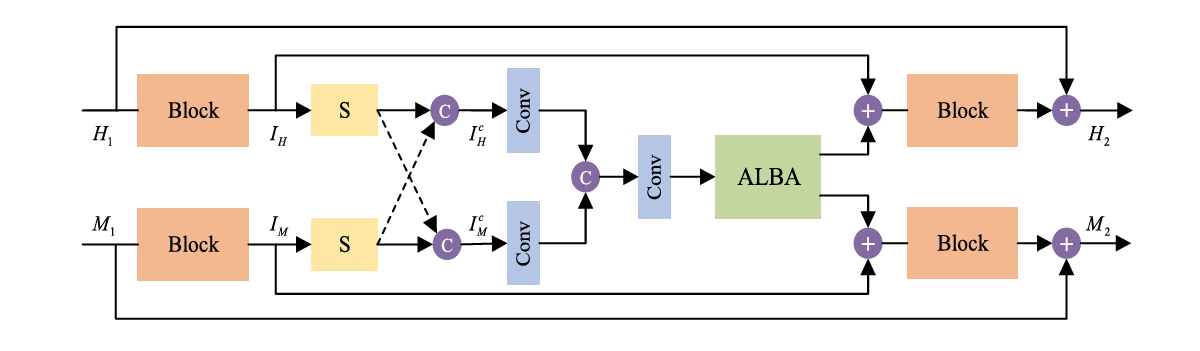
Fig. 4. Separation-and-aggregation unit (SAU)
In the coarse stage, three bands are used to perform the SR task. The model only focuses on the adjacent bands and ignores the relatively distant bands. In addition, CoarseNet only generates the general structure for LR HSI; however, it cannot effectively describe image-specific details, such as LR HSI with unknown degeneration. To capture more spectral knowledge and learn image-specific details, these coarse super-resolved bands
Dual-Stage Test Algorithm for HSI SR
Input: Given image
$I$ , trained coarse model parameter$\theta_C$ , scale factor$s$ , and number of iterations$Q$
Output: Super-resolved image$I^{SR}$
Obtain corresponding RGB image$Y$ by 1 ;
Generate LR image$Z$ by downsampling$I$ using different blur kernels and add Gaussian noise ;
Load coarse model parameter$\theta$ with$\theta_C$ ;
$I^{CR} = \mathcal{C}(s, Y, G(i); \theta_C)$ ;
Randomly initialize fine model parameter$\sigma$ , and set$q = 1$ ;
for$q \leq Q$ do
Evaluate$\mathcal{L}_ \mathcal{F}$ by 17 ;
Update$\sigma$ according to$\mathcal{L}_ \mathcal{F}$ ;
$q \gets q + 1$ ;
end
return$I^{SR} = \mathcal{F}(s, Y, I^{CR}; \sigma_ \mathcal{F})$
PyTorch, NVIDIA GeForce GTX 3090 GPU.
- Python 3 (Recommend to use Anaconda)
- PyTorch >= 1.0
- NVIDIA GPU + CUDA
- Python packages:
pip install numpy opencv-python lmdb pyyaml - TensorBoard:
- PyTorch >= 1.1:
pip install tb-nightly future - PyTorch == 1.0:
pip install tensorboardX
- PyTorch >= 1.1:
Four public datasets, i.e., CAVE, Harvard, Chikusei and Sample of Roman Colosseum are employed to verify the effectiveness of the proposed SFPN.
-
CAVE and Harvard: 80% images are randomly selected as training set and the rest as test set.
-
Chikusei: We crop the top left of the HSI (2000 × 2335 × 128) as the training set, and other content of the HSI as the test set.
-
Sample of Roman Colosseum We select the top left of the LR HSI (209 × 658 × 8) and the corresponding part of HR RGB image (836 × 2632 × 3) to train, and the remaining part of the dataset is exploited to test.
-
For the CAVE and Harvard datasets, the spectral response function of Nikon D700 camera is used to synthesize HR RGB image Y. Using another dataset, Chikusei, we crop the training set into nonoverlapping image with 200 × 194 × 128. Since the number of training set is less, 64 patches are randomly cropped on each image. Each patch is augmented by random flip, rotation, and roll.
-
Clone this repository:
git clone https://github.com/qianngli/SFPN.git cd SFPN -
Install PyTorch and dependencies from http://pytorch.org.
-
You could download the pre-trained model from HERE.
-
Remember to change the following path to yours:
SFPN/fine.pyline 124, 136.SFPN/noDU_Train.pyline 35, 39.
-
With respect to experimental setup, we select the size of convolution kernels to be 3 × 3, except for the kernels mentioned above. Moreover, the number of these kernels is set to 64.
parser.add_argument('--n_feats', type=int, default=64, help='number of feature maps') -
Following previous works, we fix the learning rate at 10^(−4), and its value is halved every 30 epoch.
parser.add_argument("--lr", type=int, default=1e-4, help="lerning rate") parser.add_argument("--step", type=int, default=30, help="Sets the learning rate to the initial LR decayed by momentum every n epochs") -
To optimize our model, the ADAM optimizer with β1 = 0.9 and β2 = 0.99 is chosen.
we also use the ADAM optimizer to learn parameters. The learning rate is fixed as 5^−5 in our study.
You can train or test directly from the command line as such:
python train.py --cuda --datasetName CAVE --upscale_factor 4
python fine.py --cuda --model_name checkpoint/model_4_epoch_xx.pth
- To demonstrate the superiority of the proposed method, five approaches for HSI SR are used, including LTTR, CMS, PZRes-Net, MHF-net, and UAL. According to training manners, these methods can be divided into two parts, i.e., supervised and unsupervised, in which the supervised methods are LTTR and CMS, and the rest are unsupervised. Note that LTTR and CMS need to use the spectral response function many times in the process of SR.
- To evaluate the performance, three metrics are applied, i.e., peak signal-to-noise ratio (PSNR), Structural SIMilarity (SSIM), and spectral angle mapper (SAM). Among these metrics, the higher the values of PSNR and SSIM, the better the performance. The value of SAM is small, which means the spectral distortion is lower.
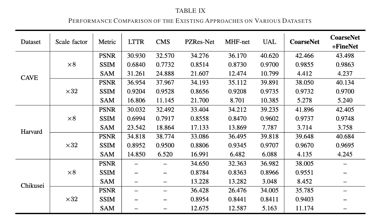
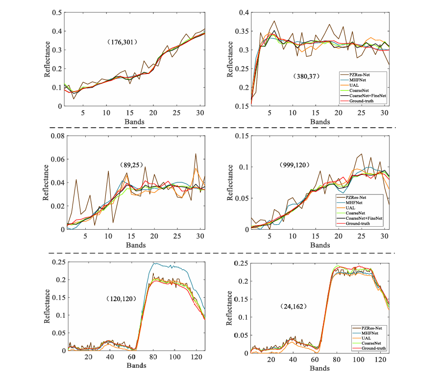
Fig. 5. Visual comparison of spectral distortion by selecting two pixels.
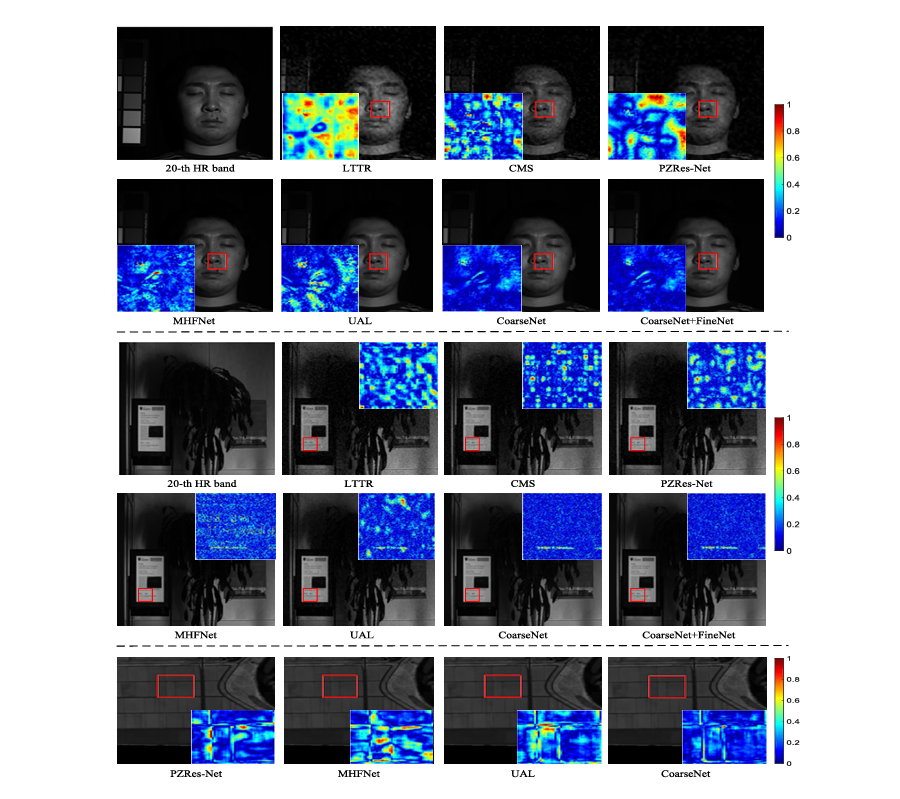
Fig. 6. Visual comparison in the spatial domain for three images. First to three lines represent the visual results of the 20th band, 20th band, and 80th band, respectively.
We apply the proposed method to a real sample located at Roman Colosseum to demonstrate its applicability.Since the HR image for this dataset is not available, we first randomly crop patch with size 36 × 36 × 8 from HSI and acquire the corresponding RGB patch with size 144 × 144 × 3. Then, the HSI patch and RGB patch are downsampled into the size 9×9× 8 and 36 × 36 × 3, respectively. Finally, the downsampled patches and original patches are exploited as training pairs. To examine the applicability, three existing models are adopted. Since there is no spectral response function, we take the above similar approach and show only partial results of the methods. Fig. 7 exhibits the super-resolved results for the existing methods. We find that some images appear smoothing or ringing results. However, the proposed CoarseNet recovers clear textures. It reveals our work can effectively tackle images in real scenes and has certain practicability.
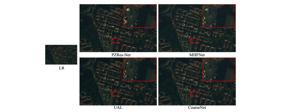
Fig. 7. Visual comparison on the real HSI dataset. We choose the 2-3-5 bands after SR to synthesize the pseudocolor image.
If you has any questions, please send e-mail to liqmges@gmail.com.