cliifs

Command Line Interface Iterated Function Systems

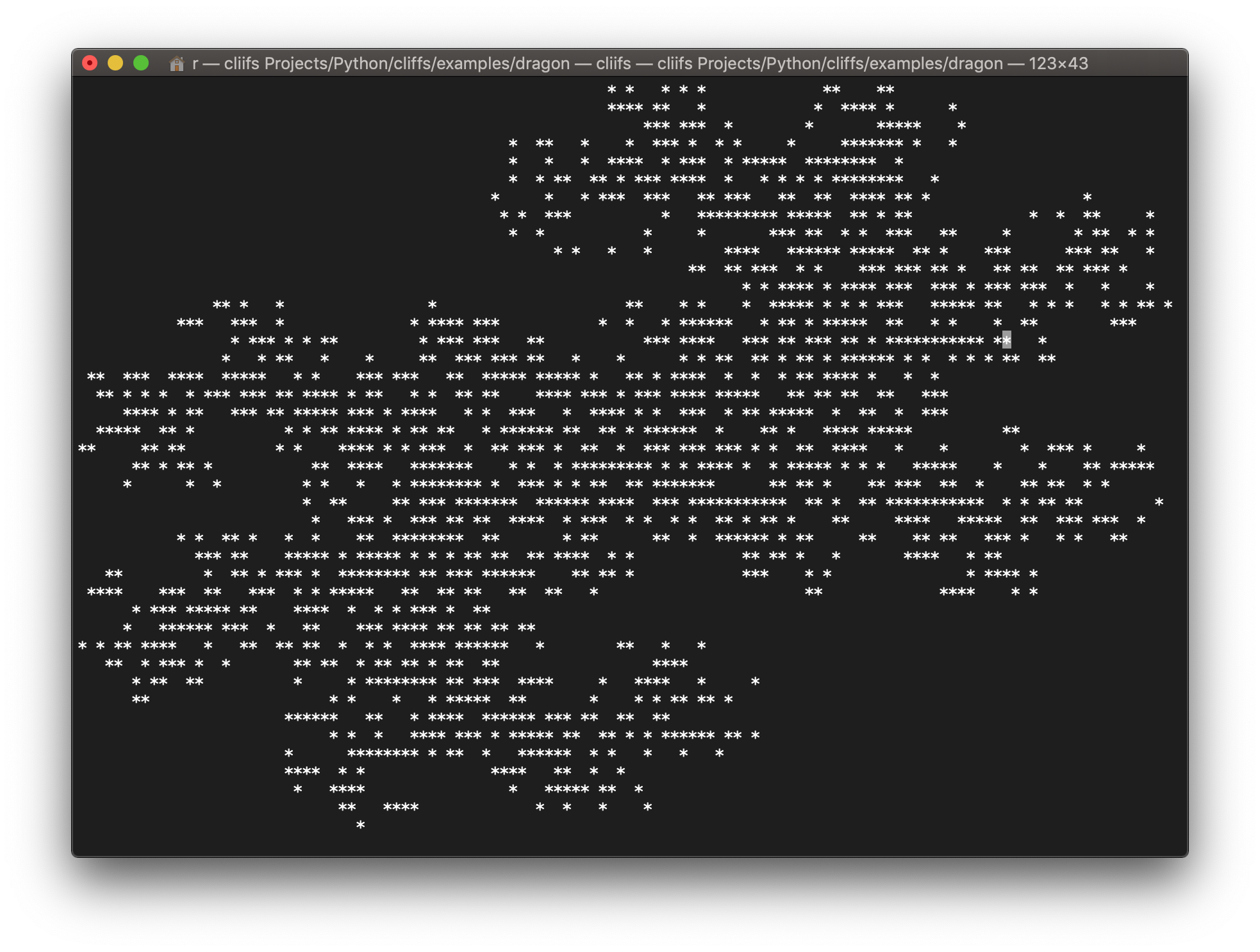
Render and view fractals, using the chaos game, from iterated functions systems right on your terminal.

Screenshots

Installation

Install via pip with pip install cliifs or download the appropriate binary from releases

How To Use

cliifs reads in a plaintext file that contains the univariate linear functions you wish to use for your IFS.

The first line must begin with either 1D or 2D.

The following lines each represent the coefficients of linear equations, and you may add as many as you like.

See below for specifics on how to write these files.

See the included examples for more details.

Invocation example

To render the IFS stored in a file called exampleFile, simply cd into the directory that contains exampleFile and run:

cliifs exampleFile

To render, with animation and color, runthe command:

cliifs exampleFile -c -a

Flags

cliifs accepts the following flags

• -h for help.
• -c to render in random colors.
• -i N to render using N iterations.
• -a to animate.
• -d D to delay each frame by D milliseconds if animating.
• -m M to set the collection of markers to be used at random.

1 Dimensional Systems

One dimensional systems are given as a test file whose first line reads simply 1D.

Each subsequent line has the form a b which represents the function f(x) = ax+b.

For example, the Cantor set, generated by f(x) = x/3+0 and g(x) = x/3+2/3, would be given as a text file with the following lines:

1D

0.333 0

0.333 0.666

2 Dimensional Systems

Two dimensional systems are given as a test file whose first line reads simply 2D.

Each subsequent line has the form a1 b1 a2 b2 c1 c2 which represents the vector function f(v) = Av+b.

In this function, A is the matrix with rows {a1, b1} and {a2, b2}, b is the vector {c1, c2} and v is the position vector {x,y}.

For example, the Sierpinski Gasket, generated by f(x,y) = (0.5x+0y, 0x+0.5y)+(0,0), g(x,y) = (0.5x+0y,0x+0.5y)+(0.5,0), and h(x,y) = (0.5x+0y,0x+0.5y)+(0.25,0.5) would be given as a text file with the following lines:

2D

0.5 0 0 0.5 0 0

0.5 0 0 0.5 0.5 0

0.5 0 0 0.5 0.25 0.5