Ames Housing

Introduction

Value Proposition

Understanding Ames

Exploratory Data Analysis

Location, Location, Zoning & Quality

[Placeholder for Neighborhood v SalePrice]

As the plot shows, neighborhoods can be ordered by the median sale price of homes which suggests which neighborhood - here a proxy for location - a home is located in is a strong indicator of price.

We see zoning as well can be ordered similar to neighborhood to give another layer to a house location. Usually similarly zoned homes are clustered together.

No need for an imposition of order - the overall quality of the home has a naturally monotonically increasing relationship with the sale price.

Price Range

Using these three features: Neighborhood, MSZoning, and OverallQual, we create a new feature called PriceRange. PriceRange is calculated by separating by quantile the median SalePrice for homes that share the same neighborhood, overall quality rating, and zoning.

As we can see in the scatter plot, the PriceRange captures some indication of overall Price. A better way to illustrate separability of the three classes is a boxplolt:

PriceRange has no information about a home's SalePrice. Yet it captures that information relatively well. We could have used more or different features in the engineering of this feature - and we will explore this topic below.

Curse of Dimensionality & Imputation

For our project, the test set was actually larger than the actual train set. This created problems when trying to do non trivial feature engineering since we - depending on our data segmentation - the test set might not have data in the bins we create for the train set.

Adding more features would have given a cleaner separability. But we also had to minimize imputation on the test set by making the feature sufficiently broad to capture the unknown price range of the test data.

We achieved a balance with the combination of Neighborhood, Zoning, and Overall Quality. These three features gave good correlation with overall price while only leaving 88 values in the test to be imputed.

Linear Models

There are four assumptions of the linear model:

1. The response is normally distributed.
2. There exists a linear relationship between the predictors, $X_i$, and the response, $Y$.
3. There are no interactions among the predictors (no multicollinearity)
4. The residual errors are independent of each other (homoscedastic)

The first three points deal with a priori assumptions on the data and target. The fourth is neccessarily model dependent.

These four points are usually taken for granted, but we decided to explore the first three and test the fourth on the Ames dataset.

Testing Assumptions

Assumption #1: Normal Distribution

Here is the distribution of the response, SalePrice:

Applying a log transfromation brings to closer to approximating a Gaussian distribution.

Assumption #2 & #3: Linearity & No Interactions

In a multicollinear model, the predictor coefficients, $\beta_i$, represent the magnitude of change in the response for a unit change in $X_i$ while holding all other $X_j$ constant.

Let's examine this idea with our new feature.

Holding PriceRange constant, we see that the relationship between Overall Quality and SalePrice for differently binned homes is highly non-linear and varies across bins.

Generalized Additive Model (GAM)

A GAM is a more generalized linear model in which the response is allowed to not only depend on sums of linear functions - but on any smooth function of the predictor variables.

Formally, the model can be expressed as:

$$g(E(Y)) = \beta_0 +f_1(X_1) + f_2(X_2) + ... + f_p(X_p)$$

Where the $f_i$ are smooth functions of the predictors, $X_i$.

By combining basis functions a GAM can represent a large number of functional relationships (to do so they rely on the assumption that the true relationship is likely to be smooth, rather than wiggly).

Motivation

The reason we chose to explore this class of models was to investigate the performance of a model that didn't make an a priori assumptions of linearity. In fact, a GAM can be used to reveal and estimate non-linear effects between the predictors on the dependent variable.


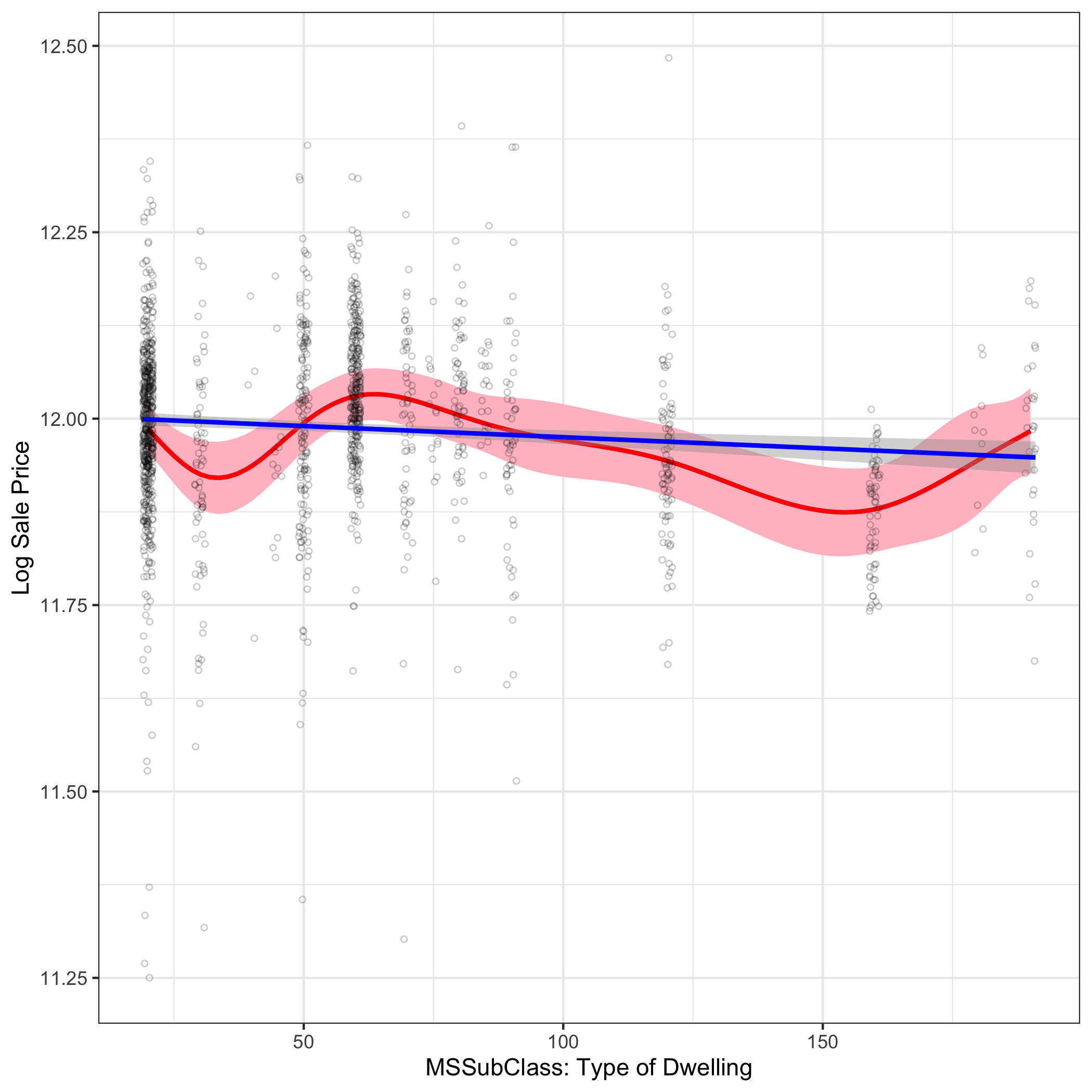
Continuous Linear	Ordinal Nonlinear
	

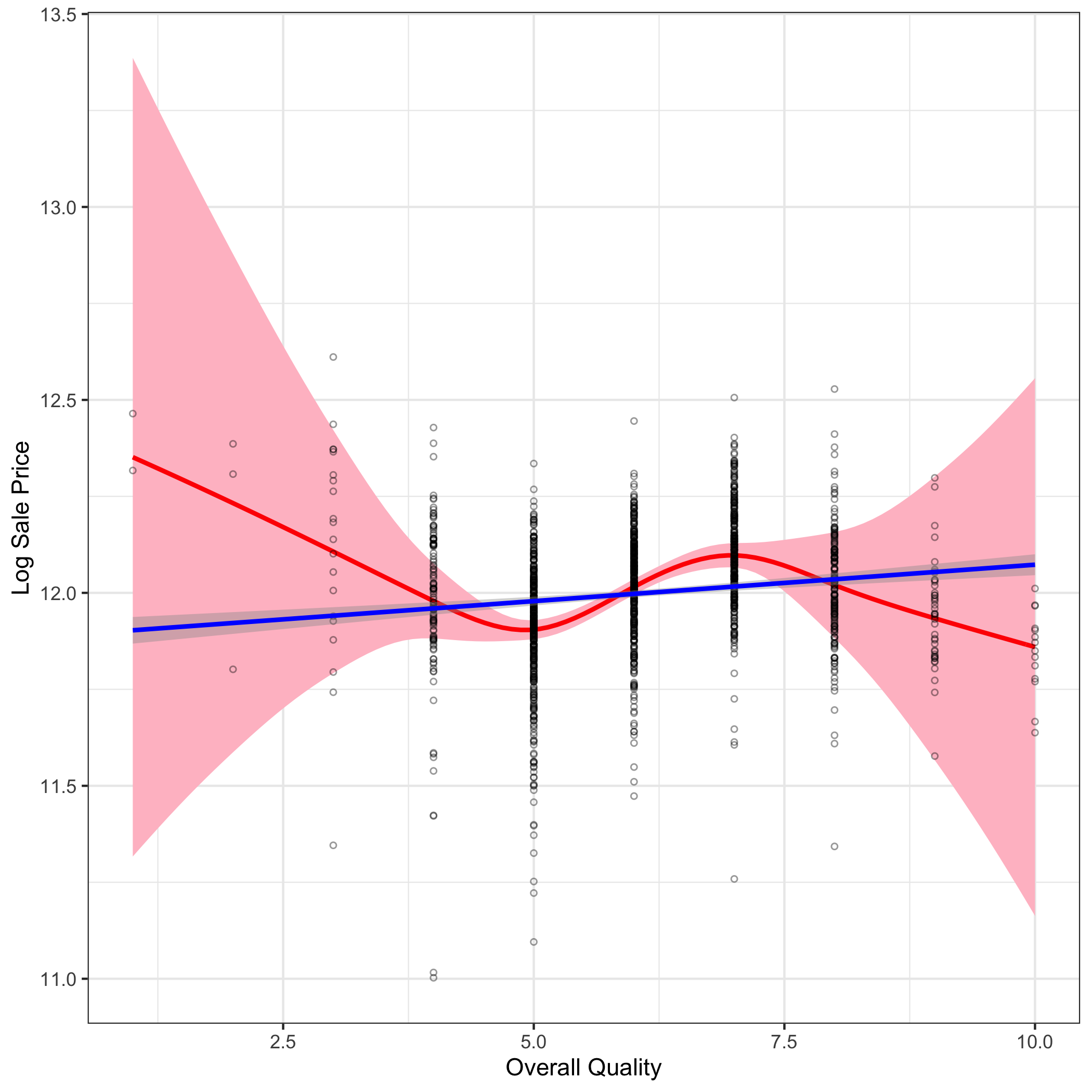
For comparison here's how closely the GAM captured the nonlinear relationship between the Overall Quality - broken out by PriceRange - and the log of the Sale Price.

Evaluation of Performance

GAM v Linear

Both models seem to underperform for low income homes with the noticable dispersion of blue points in the lower left side of both plots.

The residual plots show this more starkly. Plotted are the model residuals for both a GAM and a linear model. Most of the residuals reside within the 95% confidence band - denoted by the dashed black line. However we notice a higher proportion of low income homes (relative to middle and high) that reside outside of the band.

Size of each residual scales with magnitude

Overall these findings shows similar performance as a linear model - with many features truly exhibiting approximately linear relationships with the predictor. There is underperformance, but this is likely indicative of the common limited feature set we used for both GAM and LM.

Now that we've laid and justified the appropriate groundwork for a linear model, let's start adding features.

Ridge

Lasso

XGBoost

Conclusion

Future Work