Refactor overline function for sf objects

[Robinlovelace]

Currently overline.sf() simply wraps overline.sp(). It converts the sf object into a Spatial object before running overline.sp(), then converts it back into an sf object. This is inefficient. Furthermore there are issues with the overline.Spatial() function, e.g. as outlined in #181 and #111.

There is probably a need for aggregation via routing software such as dodgr but I think an sf-based overline() function would be useful as a number of people use it and often you have routes recorded as spatial lines. So this issue is probably overdue.

[Robinlovelace]

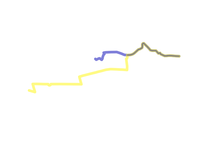
The transport ‘flow’ on any particular segment of the transport networks
is the aggregate (sum) of trips that pass through it. Finding the flow
across a transport network based on input data composed of individual
routes, is therefore an aggregation problem. It requires a more complex
solution than that provided by the aggregate() function in the base R
package stats, however, because the geometry of the output
LINESTRINGs will be fundamentally different than the input
LINESTRINGS of the routes: a route network is composed of many small
way segments, but a route is a single long LINESTRING.

Creating such a route network, with aggregated values per segment, is
the problem that the overline() function in stplanr was designed
to solve. Rather that starting from scratch and writing a geographic
algorithm from the ground-up, we will start by exploring solutions
provided by existing packages, notably sf, which provides an
interface to the GEOS library.

Let’s start simple, with just 2 lines, which have an associated amount
of flow (with illustrative values of 2 and 5 in this case):

library(stplanr)
routes_fast_sf$value = 1
sl = routes_fast_sf[2:3, ]
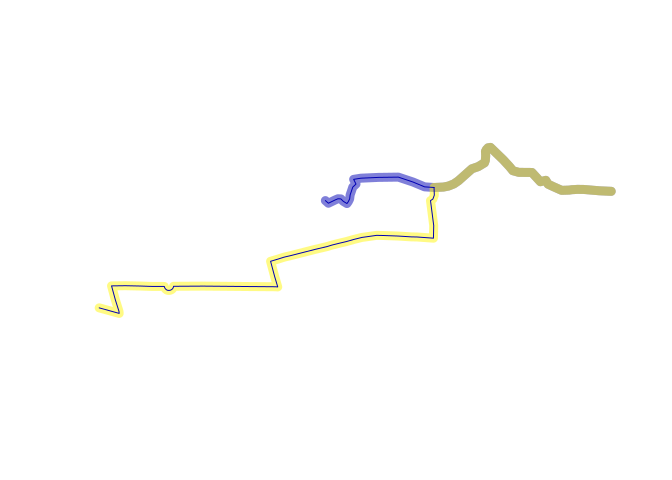
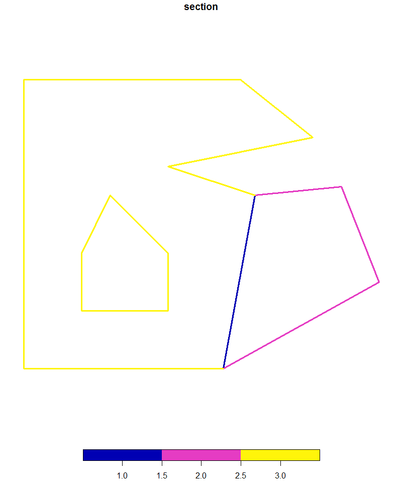
sl$value = c(2, 5)

These lines clearly have a decent amount of overlap, which can be
extracted using the function st_intersection():

sl_intersection = sf::st_intersection(sl[1, ], sl[2, ])
#> although coordinates are longitude/latitude, st_intersection assumes that they are planar
plot(sl$geometry, lwd = 9, col = sf::sf.colors(2, alpha = 0.5))
plot(sl_intersection, add = TRUE)

Furthermore, we can find the aggregated value associated with this new
segment as
follows:

sl_intersection$value = sum(sl_intersection$value, sl_intersection$value.1)

We still do not have a full route network composed of 3 non-overlapping
lines, however: the original lines need to be ‘clipped’ so that they do
not overlap with sl_intersection. This can be done as follows:

sl_seg1 = sf::st_difference(sl[1, ], sl_intersection)
#> although coordinates are longitude/latitude, st_difference assumes that they are planar
sl_seg2 = sf::st_difference(sl[2, ], sl_intersection)
#> although coordinates are longitude/latitude, st_difference assumes that they are planar
plot(sl$geometry, lwd = 9, col = sf::sf.colors(2, alpha = 0.5))
plot(sl_seg1, add = TRUE)
plot(sl_seg2, add = TRUE)

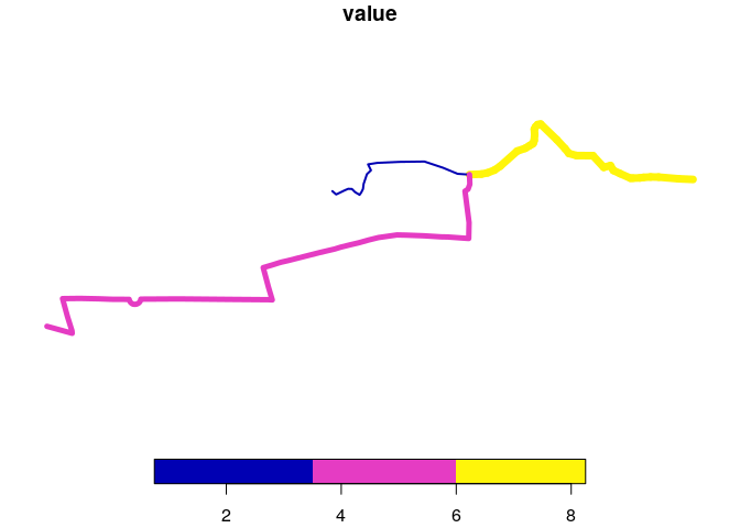
We now have all the geographic components needed for a route network.
The only remaining task is to combine them, using rbind, right? Not
quite: the following command fails:

rnet = rbind(sl_seg1, sl_seg2, sl_intersection)
#> Error in rbind.data.frame(...): numbers of columns of arguments do not match

Lesson: we need to be more careful in isolating the value to aggregate.
We will therefore run the previous stages again, but with attrib set
to the attribute we would like to aggregate over (value in this case):

attrib = "value"
attrib1 = paste0(attrib, ".1")
sl_intersection = sf::st_intersection(sl[1, attrib], sl[2, attrib])
#> although coordinates are longitude/latitude, st_intersection assumes that they are planar
sl_intersection[[attrib]] = sl_intersection[[attrib]] + sl_intersection[[attrib1]]
sl_intersection[[attrib1]] = NULL

That leaves us with a ‘clean’ object that only has a value (7) for the
attribute column name we want (value).

On this basis we can proceed to create the other segments, keeping only
the column we’re interested in. To save time and typing, we’ll create
both segments in a single command:

sl_seg = sf::st_difference(sl[attrib], sf::st_geometry(sl_intersection))
#> although coordinates are longitude/latitude, st_difference assumes that they are planar
rnet = rbind(sl_intersection, sl_seg)

It worked! Now we’re in a position to plot the resulting route network,
with ‘width’ proportional to the flow along each segment:

plot(rnet, lwd = rnet$value)

A benchmark

To test that the method is fast, or is at least not slower than the
original overline() function, at least for this task, we’ll package-up
the method in a new function:

overline_sf2 = function(sl, attrib) {
  attrib = "value"
  attrib1 = paste0(attrib, ".1")
  sl_intersection = sf::st_intersection(sl[1, attrib], sl[2, attrib])
  sl_intersection[[attrib]] = sl_intersection[[attrib]] + sl_intersection[[attrib1]]
  sl_intersection[[attrib1]] = NULL
  sl_seg = sf::st_difference(sl[attrib], sf::st_geometry(sl_intersection))
  rnet = rbind(sl_intersection, sl_seg)
  return(rnet)
}

If you are new to scripts/algorithms/functions, it may be worth taking a
look at the new
Algorithms chapter
in Geocomputation with R. Now the method has been put in a function, we
can compare its performance with the per-existing overline() function
for comparison:

system.time({overline(sl, attrib = "value")})
#>    user  system elapsed 
#>   0.049   0.000   0.049
system.time({overline_sf2(sl, attrib = "value")})
#> although coordinates are longitude/latitude, st_intersection assumes that they are planar
#> although coordinates are longitude/latitude, st_difference assumes that they are planar
#>    user  system elapsed 
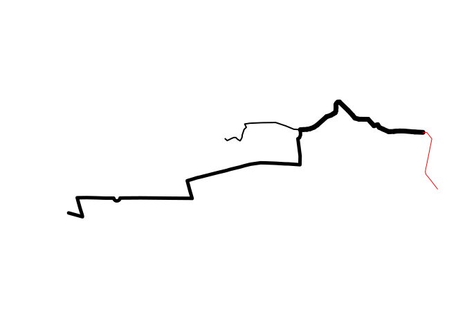
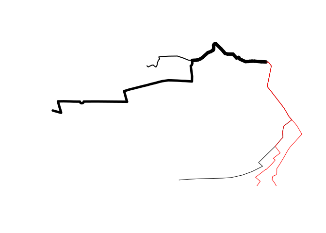
#>   0.033   0.000   0.033

The results are not Earth-shattering: the new function seems to be
around the same speed as the original, if a little faster. This is great
news, but remember: the new function only works on 2 lines so is much
simpler.

Dealing with many lines

The above method worked with 2 lines but how can it be used to process
many lines? Clearly the same function could be implemented on another
line, but it would need to work from the 3 lines of the newly created
rnet object rather than the original 2 routes. Let’s introduce a
3^rd route into the equation, that does not intersect with
this newly created rnet object:

sl3 = routes_fast_sf[4, ]
rnet = overline_sf2(sl)
#> although coordinates are longitude/latitude, st_intersection assumes that they are planar
#> although coordinates are longitude/latitude, st_difference assumes that they are planar
plot(rnet$geometry, lwd = rnet$value)
plot(sl3, col = "red", add = TRUE)

In this case the method of adding to rnet is simple: just add the
entirety of the line to the rnet object:

rnet3 = rbind(rnet, sl3[attrib])
plot(rnet3$geometry, lwd = rnet3$value)

This works fine. In fact it works better than the original overline
function because it does not add the value of the existing thickest line
in the previous figure onto the new line, a problem associated with
overline.sp() that is illustrated in the following code chunk and
resulting figure:

sl1_3 = as(routes_fast_sf[2:4, ], "Spatial")
rnet3_sp = overline(sl1_3, attrib = "value")
plot(rnet3_sp, lwd = rnet3_sp$value)

A question that arises from the previous example is this: what if the
next line intersects with the route network? It is no longer possible to
simply add together two values. This can be illustrated by introducing 2
more lines:

sl4_5 = routes_fast_sf[5:6, ]
plot(rnet3$geometry, lwd = rnet3$value)
plot(sl4_5$geometry, col = "red", add = TRUE)

Both the new lines intersect with the newest part of the route network.
This means that we cannot simply rbind() them to it as we did for
sl3. They need to be dealt with separately.

Before we deal with them, it’s worth taking some time to consider what
we mean by ‘intersect’. Intersection is actuall a specific type of
geometric relation between 2 sets of features. We can see the type of
relation by using the function st_relate():

relations = sf::st_relate(sl4_5, rnet3)
#> although coordinates are longitude/latitude, st_relate assumes that they are planar
relations
#>      [,1]        [,2]        [,3]        [,4]       
#> [1,] "FF1F00102" "FF1FF0102" "FF1FF0102" "1F1F00102"
#> [2,] "FF1F00102" "FF1FF0102" "FF1FF0102" "1F1F00102"
unique(as.vector(relations))
#> [1] "FF1F00102" "FF1FF0102" "1F1F00102"

This shows us something important: although 2 elements (1 and 4) of
rnet relate in some way to the new lines, only the 4^th
feature has a linear, overlapping relation with it. That relation is
1F1F00102 which, as far as I can tell, is not a named spatial
predicate
(FF1F00102 means ‘intersects and touches’ but does not have a linear
overlap). This relation is what we need to decide whether or not to
simply bind a new feature to the growing rnet, whether we need to
break it up (or at least part of it) into smaller lines before doing so
(it also raises the wider question of which order should we do things).

In the simple case of whether to simply bind the next line (4) onto
rnet3 the answer is simple now we know the string code associated with
linear overlaps. First we’ll test it on the previous example of sl3
and the original rnet composed of 3 features:

relate_rnet_3 = sf::st_relate(rnet, sl3, pattern = "1F1F00102")
#> although coordinates are longitude/latitude, st_relate_pattern assumes that they are planar
relate_rnet_3
#> Sparse geometry binary predicate list of length 3, where the predicate was `relate_pattern'
#>  1: (empty)
#>  2: (empty)
#>  3: (empty)
any(lengths(relate_rnet_3))
#> [1] FALSE

The FALSE meant there was no linear overlaps. So we simply used
rbind(). When we ask the same question of rnet3 and sl4, however,
the answer is TRUE:

sl4 = sl4_5[1, ]
relate_rnet_4 = sf::st_relate(rnet3, sl4, pattern = "1F1F00102")
#> although coordinates are longitude/latitude, st_relate_pattern assumes that they are planar
relate_rnet_4
#> Sparse geometry binary predicate list of length 4, where the predicate was `relate_pattern'
#>  1: (empty)
#>  2: (empty)
#>  3: (empty)
#>  4: 1
any(lengths(relate_rnet_4))
#> [1] TRUE

How to proceed? We need to avoid rnet objects containing any
overlapping lines. Because sl4 overlaps with part of rnet3 we will
need to remove the overlapping line, run the overline_sf2() function,
and then re-combine the result with the pre-existing route network
object. We can split-up the rnet3 object into overlapping and
non-overlapping features as follows:

sel_overlaps = lengths(relate_rnet_4) > 0
rnet_overlaps = rnet3[sel_overlaps, ]
rnet3_tmp = rnet3[!sel_overlaps, ]

We can check that there is only one overlapping feature as follows:

nrow(rnet_overlaps)
#> [1] 1

And we can proceed to join the two features together using our new
function:

rnet_overlaps4 = overline_sf2(rbind(rnet_overlaps, sl4[attrib]))
#> although coordinates are longitude/latitude, st_intersection assumes that they are planar
#> although coordinates are longitude/latitude, st_difference assumes that they are planar

Adding this back to the rnet3 object results in an larger rnet
object incorporating all the value and geometry column data we have
so far:

rnet = rbind(rnet3_tmp, rnet_overlaps4)
plot(rnet$geometry, lwd = rnet$value)

[mpadge]

Profound stuff for a Saturday evening, and immediately prompted this dodgr issue. Thanks for the inspiration!

[mdsumner]

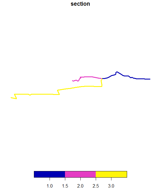
Re the "3 non-overlapping lines" part, this is exactly what ARC is meant to do - but it's totally broken for lines atm (it assumes a trick about closing polygons, but it works from a sequential model rather than edges, so needs a revisit overall).

(@Robinlovelace I haven't looked in detail at the rest of your post! )

Here's a purely SC approach. We end up with a nested column identifying which object/s each section comes from (I haven't labelled section well, and here the object_ id is the rownames of the original object, which I'm reviewing anyway).

library(stplanr)
routes_fast_sf$value = 1
sl = routes_fast_sf[2:3, ]
sl$value = c(2, 5)


library(silicate)
sc <- SC(sl)


## 3 non-overlapping lines
library(dplyr)
segments <- sc$object_link_edge %>% group_by(edge_) %>% tally() %>%  
  split(.$n)  %>% purrr::map(~inner_join(.x, sc$object_link_edge) %>% 
                               inner_join(sc$edge) %>% 
                               inner_join(sc$vertex, c(".vx0" = "vertex_")) %>% 
                               transmute(object_, .vx1, x0 = x_, y0 = y_, n) %>%   ## limit to next vertex, and this vertex values
                               inner_join(sc$vertex, c(".vx1" = "vertex_")) %>%  ## get last vertex values
                               transmute(object_, x0, y0, x1 = x_, y1 = y_, n)) %>% 
  bind_rows(.id = "section")



mk_edge   <- function(x) {
  ## one row, one segment
  sf::st_linestring(matrix(unlist(x[c("x0", "x1", "y0", "y1")]), ncol = 2))
}
mk_nest_sf <- function(x) {
  sf::st_sf(objects = tidyr::nest(x["object_"] %>% distinct(), .key = "object_"), 
                                  geometry = sf::st_union(sf::st_sfc(purrr::map(purrr::transpose(x), mk_edge))))
}

## split the 1s by object
## combine the 2s
a <- rbind(mk_nest_sf(segments %>% dplyr::filter(n == 2)), 
      do.call(rbind, purrr::map(segments %>% dplyr::filter(n == 1) %>% split(.$object_), mk_nest_sf)))
a$section <- seq_len(nrow(a))          
plot(a %>% dplyr::select(- object_), lwd = 3)

Each section is separate, and knows what object it came from

 a$object_
[[1]]
# A tibble: 2 x 1
  object_
  <chr>  
1 2      
2 3      

[[2]]
# A tibble: 1 x 1
  object_
  <chr>  
1 2      

[[3]]
# A tibble: 1 x 1
  object_
  <chr>  
1 3      

This is exactly the same plane partitioning idea used by the spacebucket - it's what Eonfusion called "fusion" and used this simplicial complex approach as silicate does. There's absolutely no dealing with fuzzy data, but that is best done independently IMO).

[mdsumner]

it works with minimal_mesh and inlandwaters (I think).

An interesting thing with this one is it's essentially grouped any path to the object it came from unless it's a shared boundary, which is fair - in reality we won't be turning back into sf like this until we're done with other tasks.

and one more with gibble::hsh$poly

This is exactly what I need to fix ARC

[mdsumner]

I'm only deal with "occurs once" or "occurs twice" cases, which is the basic deal with polygon layers - for use in what overline is doing it will have to map over n in mk_nest_sf(segments %>% dplyr::filter(n == ...)) so I'll have to think about that

[Robinlovelace]

Interesting stuff. Maybe at some time I'll have to refactor the function again, to support SC objects. Suspect it will be easier though by the looks of it. Thanks for the examples, lots of food for thought in there!

[mdsumner]

It's great, I never really had such clear and clean overlaying examples before - this a perfect test case and made me realize many things. The info is all in the object link table, we don't want to need sf to reconstruct paths from arbitrary edges!

[Robinlovelace]

Regarding next steps on my evolving overline_sf() function do you have any specific suggestions? As the examples show, it's fine up to routes_fast_sf[1:6, ] but the 7^th^ (clearly unlucky) line makes the function produce borked results. Any assistance very much appreciated (thinking: getting it working with sf will provide good use case for benchmarking SC and may be a good example of when new spatial class definitions are useful).

[Robinlovelace]

Heads-up @mem48 here's the PR that presents a methodology to do this: https://github.com/ropensci/stplanr/blob/refactor-overline/vignettes/overline.Rmd

Will be interesting to see how the 'split into single 2 point lines' method compares.

[mem48]

I promised to look at this for 20 -minute and spent slightly longer.

My method is fairly simple to explain.

1. Split every line into straight segments
2. Find duplicated segments and add their values together

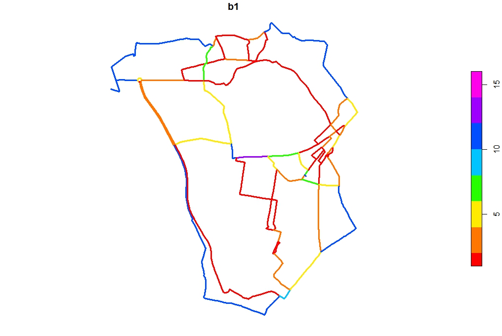
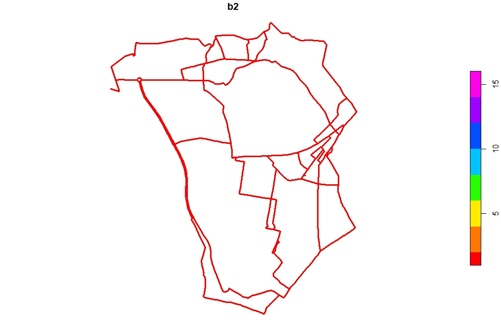
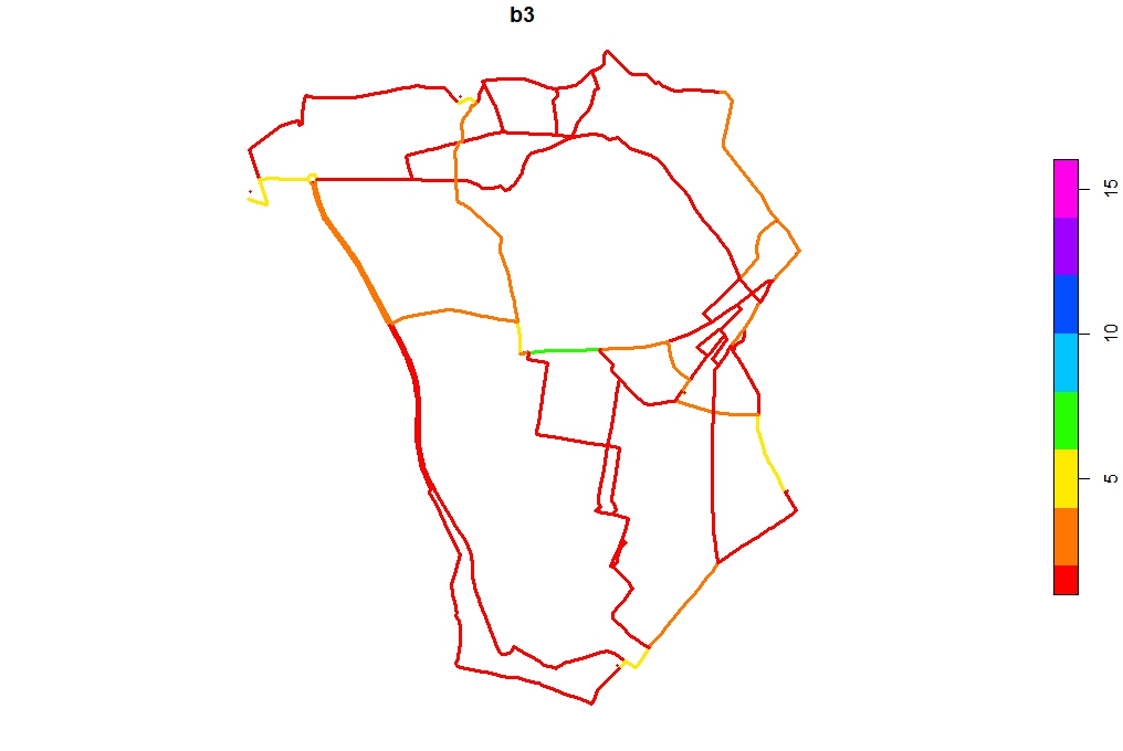
The logic being that duplicate checking is fast and easy, the downside is that you end up with many short lines rather than a few long lines that are only split when the value changes.

Two functions:

# Convert linestrings to many straight lines
line2segments = function(x){
  c1 = st_coordinates(x) # Convert SF to matrix
  l1 = c1[,3] # Get which line each point is part of
  l1_start = duplicated(l1) # find the break points between lines
  l1_start = c(l1_start[2:length(l1)],FALSE)
  seqs = seq(1,length(l1),1)[l1_start] # Make list of linestrings
  geoms = lapply(seqs, function(y){st_linestring(c1[c(y,y+1),c(1,2)])})
  geoms = st_as_sfc(geoms, crs = st_crs(x))
  dat = x # extract attributes
  st_geometry(dat) = NULL
  dat = as.data.frame(dat)
  dat = dat[l1[l1_start],, drop = FALSE] # repeate attriibutes
  st_geometry(dat) = geoms # put together
  return(dat)
}

# Overlay duplicated lines
overline_malcolm = function(x, attrib){
  if(all(st_geometry_type(x) != "LINESTRING")){
    message("Only LINESTRING is supported")
    stop()
  }
  x = x[,attrib]
  x_split = line2segments(x) # Split into segments
  x_dupe = duplicated(x_split$geometry)
  times = unique(x_split[,"geometry", drop = FALSE]) # make lookup table
  times$id = seq(1,nrow(times))
  x_split$matchingID = times$id[match( x_split$geometry, times$geometry)]
  x_group = x_split[,c("matchingID",attrib)]
  st_geometry(x_group) = NULL 
  x_group = x_group %>%
    group_by(matchingID) %>%
    summarise_all(funs(sum))
  x_nodupe = x_split[!x_dupe,]
  x_nodupe$value = NULL
  x_nodupe = left_join(x_nodupe,x_group,"matchingID" )
  x_nodupe = x_nodupe[,attrib]
  return(x_nodupe)
}

Some basic tests:

library(stplanr)
library(sf)
library(dplyr)
routes_fast_sf$value = 1
sl = routes_fast_sf[2:5, ]
system.time({b1 = overline(sl, attrib = "value")})
# user  system elapsed 
#   1.09    0.02    1.11
system.time({b2 = overline_sf2(sl, attrib = "value")})
# user  system elapsed 
#   0.04    0.00    0.03 
system.time({b3 = overline_malcolm(sl, attrib = "value")})
# user  system elapsed 
#  0.23    0.00    0.25 

So it is faster than overline but not as fast as robin's new method. But each method give a different results

pal = c("#FF0000FF", "#FF7600FF", "#FFEB00FF" ,"#27FF00FF" ,"#00C4FFFF",
"#004EFFFF" , "#9D00FFFF", "#FF00EBFF" )
breaks = c(1,2,4,6,8,10,12,14,16)
plot(b1, main = "b1", lwd = 3, pal = pal, breaks = breaks)

plot(b2, main = "b2", lwd = 3, pal = pal, breaks = breaks)

plot(b3, main = "b3", lwd = 3, pal = pal, breaks = breaks)

I've done a little manual checking and I think my method is giving the correct results but needs some oversight.

[Robinlovelace]

That doesn't look like the first 4 lines but all of them! In any case this looks very promising and a good starter for a new implementation, potentially that is well suited to parallelisation in a lower level language like C++/rust.

[Robinlovelace]

overline_malcolm() nice function name!

[mem48]

@Robinlovelace done more work on this as part of the PCT Phase 3. https://github.com/mem48/pct-raster-tests/blob/master/R/overline.R The code has changed a lot from my earlier example, around improving performance on large datasets and simplifying the geometry at the end to fewer longer lines.

[Robinlovelace]

Latest: I will test the new function and incorporate from here https://github.com/mem48/pct-raster-tests

[mem48]

https://github.com/mem48/pct-raster-tests/blob/master/R/overline.R contains the function called overline_malcolm2 (working title) which is the one in need of checking. There is one known bug when a route stops halfway down a segment, then the overlapping segments do not match and the function does not identify the overlap

[Robinlovelace]

Here are some benchmarks for overline btw:

Dataset with 60,000 lines in 214s:

> system.time({
+   rnet = overline2(rf_i, scenarios)
+ })
2019-03-29 13:56:10 constructing segments
2019-03-29 13:56:13 transposing 'B to A' to 'A to B'
   |++++++++++++++++++++++++++++++++++++++++++++++++++| 100% elapsed = 17s
2019-03-29 13:57:31 removing duplicates
2019-03-29 13:57:57 restructuring attributes
2019-03-29 13:58:15 building geometry
   |++++++++++++++++++++++++++++++++++++++++++++++++++| 100% elapsed = 19s
2019-03-29 13:58:37 simplifying geometry
2019-03-29 13:59:40 rejoining segments into linestrings
   user  system elapsed 
206.330   8.000 214.617 

[Robinlovelace]

~ 300 lines per second. Not bad. That suggests for 2 million routes over the UK it will be around 2 hours:

> (2000000 / 300 ) / (60 * 60)
[1] 1.851852