If you are comfortable managing and installing your own python environments and packages you are free to do so. The following instructions use conda because several of our dependencies rely on C-libraries to be preinstalled.
First, let's create a blank environment called ilamb-watersheds and activate it.
conda create --name ilamb-watersheds
conda activate ilamb-watersheds
The ILAMB package v2.6 is already built in the conda-forge channel. We need to make sure that this channel is added. If you use conda, you probably have already done this, but it does not hurt to run it again.
conda config --add channels conda-forge
conda config --set channel_priority strict
Then we can install ILAMB.
conda install ILAMBThe capabilities we are presenting today have been written for this tutorial and are not yet into a release of ILAMB. So we will install ILAMB again on top of the conda build but this time directly referencing the master branch from github with the watershed extras. Navigate to some location where you keep source code and then:
git clone https://github.com/rubisco-sfa/ILAMB.git
cd ILAMB
python -m pip install '.[watershed]'
The watershed extras installs additional packages that we need to handle geographic projections and query the USGS data servers. By including them as extras, more traditional ILAMB users can avoid installing packages they do not need. Note that depending on your system, you may also need to install wget and gdal. These can also be added with conda:
conda install wget
conda install gdal
Finally we can test that all of this worked by running:
python -c "import ILAMB; print(ILAMB.__version__)"If you get a numeric 2.6, then your ILAMB package should be setup correctly and you are ready to go!
This tutorial is meant to work on the raw output from the ELM run conducted in the first part of this tutorial. If you were not able to run the model or were not present, we have bundled a version of the output that you can download and use. Please note that to keep the size managable, we have removed most of the variables.
If you would like to use the data from your run you either need to:
- Move your ELM output out of the docker area (preferred).
- Spin up the docker instance and install conda and ILAMB within. Note that, similar to having to reclone the
OLMTevery time you launch the docker image, you will have to reinstall conda and ILAMB each time you spin up.
mkdir tutorial
cd tutorial
mkdir MODELS
cd MODELS
If you are using your own model output, then this is where we need to place your h0 and h1 netCDF files from the docker image. Note that you can simply provide a link to the folder where you have the files downloaded if you prefer not to move them. Alternatively, if you are using the sample output that we have prepared for you, then here is where we need to expand the tar-ball.
wget https://www.ilamb.org/~nate/ELM.tgz
tar -xvf ELM.tgz
Next, we need to get some reference dataset to make a comparison to the ELM output. In standard ILAMB, you would download our large collection. However, these datasets are at a half degree resolution and are not interesting to compare to the ELM watershed run.
NASA has MODIS data available for download on their Aρρears (Application for Extracting and Exploring Analysis Ready Samples) portal. This data portal allows you to specify a polyline representing your watershed, and then download MODIS data at 8 day resolution for just that area. To download your own data, you will need a free login with that website.
As requests to Aρρears are not instantaneous, we have already made a request for MODIS gpp over the American River watershed (actually a larger area) and have processed this data to make suitable for ILAMB analysis using this script. You can simply download the result from our site following the steps below.
cd ..
mkdir DATA
cd DATA
mkdir MODIS
cd MODIS
wget https://www.ilamb.org/~nate/AmericanRiverWashington.nc
At this point, we are ready to setup our ILAMB analysis. As a check, your data should look like this:
./tutorial
├── DATA
│   └── MODIS
│       └── AmericanRiverWashington.nc
└── MODELS
    └── ELM
        ├── 20230411_ini_hcru_hcru_ICB20TRCNPRDCTCBC.elm.h0.1980-01.nc
        ├── 20230411_ini_hcru_hcru_ICB20TRCNPRDCTCBC.elm.h0.1980-02.nc
        ├── ...
        ├── 20230411_ini_hcru_hcru_ICB20TRCNPRDCTCBC.elm.h0.2014-11.nc
        ├── 20230411_ini_hcru_hcru_ICB20TRCNPRDCTCBC.elm.h0.2014-12.nc
        ├── 20230411_ini_hcru_hcru_ICB20TRCNPRDCTCBC.elm.h1.1980-01-01-00000.nc
        ├── ...
        └── 20230411_ini_hcru_hcru_ICB20TRCNPRDCTCBC.elm.h1.2015-01-01-00000.nc
where I have left ... just to shorten the list of files present in the printed directory.
In order to run the ILAMB analysis we need to signal to ILAMB (1) the reference datasets we want to compare against and (2) the models that are going to be part of the study.
To setup the reference datasets, add a file to the tutorial directory called watersheds.cfg and paste the following text inside.
[h1: USWatersheds]

[h2: AmericanRiverWashington]

[MODIS_gpp]
variable = "gpp"
source = "DATA/MODIS/AmericanRiverWashington.nc"
plot_unit = "g m-2 d-1"
table_unit = "g m-2 d-1"
cmap = "Greens"
ILAMB will read this configure file and use it organize an analysis. The tags inside of the h1 and h2 are just organizational headings. Let's focus on the contents of the [MODIS_gpp] tag.
- The text between the brackets
MODIS_gppis how the dataset will appear on the website once the comparison is done. You may choose any text you like here as long as they are valid characters in file and directory names. - We set the
variableto begpp. It is our convention to follow CMIP/CMOR standards when possible. If you are familiar with the ELM output, you may realize that the variable therein isGPP. More on this later. - We set the
sourceto be the location of the reference data relative to this top level directory. This makes your configure file portable to other systems and something you can share with others and build on collectively. - ILAMB handles units internally using a python wrapper (
cf_units) around the UDUnits library. So here we can specify how we want all the models' units to appear in the final output and ILAMB will make the conversions internally. - Finally we set a colormap. This needs to be one of
matplotlib's colormaps and we have selectedGreenshere because we find it intuitive when thinking ofgpp.
At this point, we need to set an environment variable which ILAMB will use internally to prepend to the source path given in your file. From the top level tutorial directory, run:
export ILAMB_ROOT=./In order to setup our models, we will create another file called models.yaml and paste inside it the following:
ELM:
  type: E3SMResult
  color: '#ff7f0e'
  path:
   - MODELS/ELM
  synonyms:
    GPP: gpp
  unit_replace:
    gC: g
I apologize for having multiple file types to setup ILAMB. This code has been around now for 7 years and technology continues to evolve. In the future we will be transitioning to simply using yaml formats for everthing. Let's discuss the contents of each line of this file.
- The top level is the model name, that is, how you want the model to appear on the HTML output page. In this case we simply call it
ELM. - We need to give it a model type. Normally you could leave this blank and use the general ILAMB model result which works on regular lat/lon gridded output. For example, if you wanted to compare to some ELM output that has been CMORized already, you would leave this blank. For this tutorial, I have implemented a special model type
E3SMResultto handle raw output even from unstructured grids. - We can assign a color to the model. When running with multiple models, this will be the color this model appears as the line plots.
- This
pathvariable can be a list of paths of where to find model output. It can be an absolute path if your model output is located elsewhere or in some standard location, but here points to where we have copied our ELM output. - You can now define synonyms for your model. In the configure file, we used the CMOR variable
gppbut ELM usesGPP. This section signals that whengppis required of this model, useGPPinstead. This keeps you from having to run output conversion routines. In this case the difference is only case, but in general variable names might not resemble each other at all. - Many times the raw output from models does not provide a unit string that is compatible with standards. The
E3SMResultmodel object allows you to specify aunit_replacedictionary which will be applied to the unit string of any variable you try to access. In this case, we need to remove theCfromgC(grams carbon) as this is not a unit that the UDunits2 library recognizes.
We are now ready to run. When you installed ILAMB, we also installed a few ilamb-XXX commands, one of which is ilamb-run. We need to provide an argument to let it know which configure file to use --config watersheds.cfg as well as the setup information for our models --model_setup models.yaml. This should produce the following:
(ilamb-watersheds) [nate@narwhal tutorial]$ ilamb-run --config watersheds.cfg --model_setup models.yaml
                                             E3SM

Parsing config file watersheds.cfg...

                AmericanRiverWashington/MODIS_gpp Initialized

Running model-confrontation pairs...

                AmericanRiverWashington/MODIS_gpp E3SM                 Completed  0:00:05

Finishing post-processing which requires collectives...

                AmericanRiverWashington/MODIS_gpp E3SM                 Completed  0:00:02

Completed in  0:00:15
The ILAMB analysis occurs in two phases. The first phase compares all models to the reference datasets--in this case we have 1 of each and so very little took place. In our larger runs we have ~60 datasets and ~20 models and can take several hours. ILAMB will execute this work list in parallel, but we do not need this feature today. In the second phase, ILAMB looks at all the analysis intermediate files and then generates plots and html pages. If you list the tutorial directory now, you will see a _build directory has been generated.
drwxr-xr-x. 3 nate nate 4.0K Apr 21 14:41 _build
drwxr-xr-x. 3 nate nate 4.0K Apr 21 13:20 DATA
drwxr-xr-x. 3 nate nate 4.0K Apr 21 12:55 MODELS
-rw-r--r--. 1 nate nate   92 Apr 21 14:40 models.yaml
-rw-r--r--. 1 nate nate  193 Apr 21 13:46 watersheds.cfg
Inside the directory you will find a hierarchy of wepages which ILAMB generated for you. To get the top page to appear properly, you will need to emulate a http server.
cd _build
python -m http.server
You will get some text saying that the page is being served to some address like http://0.0.0.0:8000/. Click on this clink and your results will load in your browser. If you are on a remote connection, you will need to move this _build directory to some web-viewable space or locally to your computer to view. Alternatively, I have copied the output from this step here as well.
If you made it this far, congratulations! These steps illustrate the basic functionality that ILAMB provides: a means to systematically compare your model output to reference datasets. They mostly use code and methods that we have developed in the past years. In what follows we will demostrate how ILAMB can be adapted and expanded to address application needs.
For watershed comparisons, we have implemented a specialized confrontation (our term for the object which encapsulates a model-data comparison) which automatically queries USGS servers for discharge data. To set this up, add the following lines to the bottom of your watersheds.cfg file.
[USGS_mrro]
ctype = "ConfUSGS"
sitecode = "12488500"
time_start = "1980-1-1"
time_end = "2021-1-1"
This adds a special kind of confrontation, which we designate using the ctype keyword. This controls what kind of analysis is performed and can contain any custom code that a user wants to include. This confrontation is written to take in a USGS sitecode, along with a time frame, and automatically download the data needed to compare to model output. These sitecodes can be browsed on this interactive map. All that ILAMB needs is the code number and the comparison will use their interface to grab all the required data.
When used to compare against gridded data, like we have with ELM, then ILAMB will integrate the runoff variable and compare against the gauge data. For this to work, we need to add another synonym to the ELM in our models.yaml file.
  synonyms:
    GPP: gpp
    QRUNOFF: discharge
Because we are changing something about the model, we need to clear the model cache so that the additional synonym will be available in the ILAMB analysis.
rm _build/ELM.pklNow you re-run the same ilamb-run command as before. This time you will see an additional confrontation which bears the name from the USGS site AMERICAN RIVER NEAR NILE, WA.
(ilamb-watersheds) [nate@narwhal tutorial]$ ilamb-run --config watersheds.cfg --model_setup models.yaml
                                             E3SM

Parsing config file watersheds.cfg...

                AmericanRiverWashington/MODIS_gpp Initialized
                     AMERICAN RIVER NEAR NILE, WA Initialized

Running model-confrontation pairs...

                     AMERICAN RIVER NEAR NILE, WA E3SM                 Completed  0:00:31

Finishing post-processing which requires collectives...

                AmericanRiverWashington/MODIS_gpp E3SM                 Completed  0:00:02
                     AMERICAN RIVER NEAR NILE, WA E3SM                 Completed  0:00:01

Completed in  0:01:00
As before, we view the output by:
cd _build
python -m http.server
and then follow the link. Alternatively, you can view what the output should look like by following this link. If you navigate to the USGS page, you will find statistics and plots like the following:
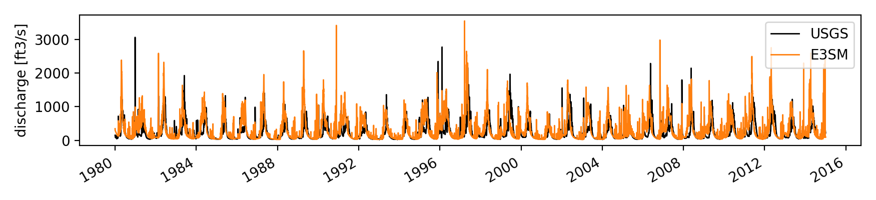
While the discharge metric for ELM looks decent, we should compare its performance to other models. We have collected results from the National Water Model (NWM), Soil & Water Assessment Tool (SWAT), and the Advanced Terrestrial Simulator (ATS). However, while each of these models has been run on their own mesh, and handles the routing of runoff, the only output we have recorded is at the outlet which corresponds to our USGS station.
We can integrate these models into ILAMB as well. First, add the output files to your collection.
cd MODELS
wget https://www.ilamb.org/~nate/point_models.tgz
tar -xvf point_models.tgz
Next, we need to add entries to our models.yaml file. There are a few key differences. This type the type of model we will use is one we have written to handle point output. This model type also requires that we provide a map between the file and the USGS sitecode. Ultimately we would rather harvest this information from the output file directly, but this will require these models making that change to embed the sitecode. Note that the variable representing discharge is different for each model. We simpy add the appropriate synonym to each model.
ATS:
  name: ATS
  type: ModelPointResult
  color: '#1f77b4'
  path:
   - MODELS/ATS
  file_to_site:
    ARW_calibrated_qetsc_wb_1997-2020.csv: '12488500'
  synonyms:
    'watershed boundary discharge': discharge

NWM:
  name: NWM
  type: ModelPointResult
  color: '#2ca02c'
  path:
   - MODELS/NWM
  file_to_site:
    NWM_streamflow_featureid24422913.csv: '12488500'
  synonyms:
    Discharge: discharge

SWAT:
  name: SWAT
  type: ModelPointResult
  color: '#d62728'
  path:
   - MODELS/SWAT
  file_to_site:
    calb_model_flow.csv: '12488500'
  synonyms:
    flow: discharge
Then we re-run the same ilamb-run command again:
(ilamb-watersheds) [nate@narwhal tutorial]$ ilamb-run --config watersheds.cfg --model_setup models.yaml
                                             E3SM
                                              ATS
                                              NWM
                                             SWAT

Parsing config file watersheds.cfg...

                AmericanRiverWashington/MODIS_gpp Initialized
                     AMERICAN RIVER NEAR NILE, WA Initialized

Running model-confrontation pairs...

                AmericanRiverWashington/MODIS_gpp ATS                  VarNotInModel
                AmericanRiverWashington/MODIS_gpp NWM                  VarNotInModel
                AmericanRiverWashington/MODIS_gpp SWAT                 VarNotInModel
                     AMERICAN RIVER NEAR NILE, WA ATS                  Completed  0:00:01
                     AMERICAN RIVER NEAR NILE, WA NWM                  Completed  0:00:01
                     AMERICAN RIVER NEAR NILE, WA SWAT                 Completed  0:00:01

Finishing post-processing which requires collectives...

                AmericanRiverWashington/MODIS_gpp E3SM                 Completed  0:00:02
                AmericanRiverWashington/MODIS_gpp ATS                  Completed  0:00:01
                AmericanRiverWashington/MODIS_gpp NWM                  Completed  0:00:01
                AmericanRiverWashington/MODIS_gpp SWAT                 Completed  0:00:01
                     AMERICAN RIVER NEAR NILE, WA E3SM                 Completed  0:00:01
                     AMERICAN RIVER NEAR NILE, WA ATS                  Completed  0:00:01
                     AMERICAN RIVER NEAR NILE, WA NWM                  Completed  0:00:01
                     AMERICAN RIVER NEAR NILE, WA SWAT                 Completed  0:00:01

Errors occurred in the run, please consult ./_build/ILAMB06.log for more detailed information

Completed in  0:00:27
This time you will see some VarNotInModel errors for MODIS gpp. This is because these point models do not have that variable available. Instead of failing, ILAMB just skips this and continues to compute on what is present. View the output as before or follow this link to a version we have cached for you.