As according to Emmanoulopoulos et al 2013, Monthly Notices of the Royal Astronomical Society, 433, 907
e.g. as Connolly, S. D., 2016, Astrophysics Source Code Library, record ascl:1602.012
The code's entry in the ASCL is available here:
(A very short research note on the creation of this code has also been published on ArXiv here: http://arxiv.org/abs/1503.06676 )
If you have questions, suggestions, problems etc. please email me at sdc1g08@soton.ac.uk
(Though please note that I am not paid to maintain or update this code, so I may not be available or able to help you in all cases and will be doing so in my own time)
Note that the main purpose of this code is the simulation of lightcurves using the Emmanoulopoulos
method with known parameters for the PSD and PDF of the desired lightcurve - functions related to
fitting these distributions are added for convenience, but the results should always be checked,
as these will not always give the best fit to the data, especially with the default parameters,
and may not work at all in some cases. The use of these functions is NOT essential to simulating
lightcurves, as best fit paramaters to any distribution using other tools can always be used instead.
To install this module, download this repository by clicking 'download zip' on the right --->'
-
unzip the file
-
run the install script in the top-level directory:
python setup.py installThis will install the code as a module so that it can be imported in any working directory, e.g. with the command:
from DELCgen import *The code uses a 'Lightcurve' class which contains all of the data and functions necessary for simulation of artificial version, and for plotting and saving. Lightcurve objects can be easily created from data using the following command:
lc = Load_Lightcurve(fileroute,tbin)They can also be created manually:
lc = Lightcurve(time,flux,errors=None,tbin)Where 'time' and 'flux' are data arrays of the lightcurve. 'Errors' is an optional array of errors on the fluxes in the lightcurve, not used for simulation. 'tbin' is the sample rate of the lightcurve, which is used in simulation.
The input file must be a text file with three columns of time, flux and the error on the flux. The lightcurve must also be binned at regular intervals. Headers, footers etc. are handled.
The code can be used to produce lightcurves with any given PSD, PDF, mean and standard deviation by passing these to a single command, e.g.:
delc = Simulate_DE_Lightcurve(PSDmodel,PSDparams,PDFmodel, PDFparams,
				tbin = 1, LClength = 1000, mean = 1, std = 0.1)
where 'PSDmodel' and 'PDFmodel' can be any function giving the distribution of the PSD and PDF, and, 'PSDparams' and 'PDFparams' are tuples containing the parameters for these distributions, e.g.:
delc = Simulate_DE_Lightcurve(BendingPL, (1.0,300,2.1,2.3,0.1),
				scipy.stats.lognorm,(0.3, 0.0, 7.4),
                                  tbin = 1, LClength = 1000, mean = 1, std = 0.1)
The result is a Lightcurve object and can therefore easily be plotted, saved etc.
NOTE that the normalisation of the periodogram of the output lightcurve will not be that of the input PSD, as it is a single realisation of limited length, unless the mean of the output lightcurve for that normalisation is known. This will not be a problem in most cases, but can be addressed by renormalising the output light curve if necessary.
Artificial lightcurves can be produced with the same PSD and PDF as a data lightcurve using the following command:
delc = datalc.Simulate_DE_Lightcurve()However, this will use the default PSD and PDF distributions and starting parameters for automatic fits, which may not be the best choice in many cases.
Lightcurves can therefore be simulated for any specific given PSD and PDF model using:
From Timmer & Koenig, 1995, Astronomy & Astrophysics, 300, 707.
tklc = Simulate_TK_Lightcurve(datalc,PSDfunction, PSDparams, RedNoiseL, aliasTbin, RandomSeed)From Emmanoulopoulos et al., 2013, Monthly Notices of the Royal Astronomical Society, 433, 907.
delc = Simulate_DE_Lightcurve(datalc,PSDfunction, PSDparams, PDFfunction, PDFparams)The lightcurve's length, mean and standard deviation of the simulated lightcurve can be changed from that of the data lightcurve by providing these values as in the example of simulating without data above.
Any function can be used for the PSD and PDF, however it is highly recommended to use a scipy.stats random variate distribution for the PDF, as this allows inverse transfer sampling as opposed to rejection sampling, the latter of which is much slower. In the case that a scipy RV function is used, however, care should be taken with the parameters, as they may not be what you expect (see below). In addition, the following functions exist in the module:
- BendingPL(v,A,v_bend,a_low,a_high,c) - Bending power law
-
MixtureDist(functions,n_args,frozen=None) - Mixture distribution CLASS for creating an object which can calculate a value from or sample a mixture of any set of functions. The number of arguments of each function must be specified. Specific parameters can also be frozen at a given value for each function, such that the resultant function does not take this parameter as an argument.
e.g. mix_model = Mixture_Dist([st.gamma,st.lognorm],[3,3],[[[2],[0]],[[2],[0],]]) produces a mixture distribution consisting of a gamma distribution and a lognormal distribution, both of which have their 3rd parameter frozen at 0. The resultant function will therefore require 4 parameters (two for the gamma distribution and two for the lognormal distribution) plus the weights of each.
The value of this function at a given value of 'x' for a given set of parameters can then be obtained using mix_model.Value(x,params), where 'params' is a list of the parameters followed by the weights of each function in the mixture distribution, e.g. [f1_p1,f1_p2,f2_p1,f2_p1,w1,w2] in this case.
The function can also be randomly sampled using mix_model.Sample(params,length=1), where 'params' is the function parameters given as described above and 'length' is the length of the resultant sample array, i.e. the number of samples drawn from the distribution.
A large number of these distributions are available and are genericised such that each can be described with three arguments: shape, loc (location) and scale. As a result, some of the parameters aren't what you might expect, and each of these three parameters are needed when using a scipy RV function in this code. These can be used in mixture distributions in the code, shown in examples below. The scipy documentation is the best place to check this, but below are examples of this in the form of the Gamma and lognormal distributions which can describe AGN PDFs well:
- For a log normal distribution with a given mean and sigma (standard deviation):
scipy.stats.lognorm.pdf(x, shape=sigma,loc=0,scale=np.exp(mean))- For a gamma distribution with a given kappa and theta:
scipy.stats.pdf(x, kappa,loc=0, scale=theta)http://docs.scipy.org/doc/scipy-0.14.0/reference/stats.html
The following commands are methods of the Lightcurve class:
- Fit_PSD() - Fit the lightcurve's periodogram with a given PSD model.
- Fit_PDF() - Fit the lightcurve with a given PDF model
The following commands are methods of the Lightcurve class:
- delc = datalc.Simulate_DE_Lightcurve() - Simulate a lightcurve with the same PSD and PDF as the data lightcurve, using the Emmanoulopoulos method.
The following commands require a model and best-fit parameters as inputs:
- tklc = Simulate_TK_Lightcurve(datalc,PSDfunction, PSDparams, RedNoiseL, aliasTbin, RandomSeed) - Simulate a lightcurve with a given PSD and PDF, using the Emmanoulopoulos method
- delc = Simulate_DE_Lightcurve(datalc,PSDfunction, PSDparams, PDFfunction, PDFparams) - Simulate a lightcurve with a given PSD and PDF, using the Timmer and Koenig method.
The following commands are methods of the Lightcurve class:
- Plot_Lightcurve() - Plot the lightcurve
- Plot_Periodogram() - Plot the lightcurve's periodogram, and PSD model if fitted
- Plot_PDF() - Plot the lightcurve's probability density function, and PDF model if fitted
- Plot_Stats() - Plot the lightcurve, its periodogram and PDF, and PSD and PDF models if fitted
The following commands take Lightcurve objects as inputs:
- Comparison_Plots(lightcurves,bins=25,norm=True) - Plot multiple lightcurves and their PSDs & PDFs
The following commands are methods of the Lightcurve class:
- Save_Lightcurve(filename) - Save the lightcurve (time and flux) as a text file
- Save_Periodogram(filename) - Plot the periodogram (frequency and power) as a text file
- time - The lightcurve's time array
- flux - The lightcurve's flux array
- errors - The lightcurve's flux error array
- length - The lightcurve's length
- freq - The lightcurve's periodogram's frequency array
- periodogram - The lightcurve's periodogram (if calculated)
- mean - The lightcurve's mean flux
- std - The lightcurve's standard deviation
- std_est - The lightcurve's estimated underlying SD (if calculated)
- tbin - The lightcurve's time bin size
- fft - The lightcurve's Fourier transform (if calculated)
- psdModel - The model used in fitting the lightcurve's periodogram
- psdFit - The fit outcome from fitting the lightcurve's PDF, including the best fitting parameters
- pdfModel - The model used in fitting the lightcurve's probability density function
- pdfFit - The fit outcome from fitting the lightcurve's PSD, including the best fitting parameters
The following commands are methods of the Lightcurve class:
- STD_Estimate() - Calculate the estimate of the underlying standard deviation (without Poisson noise), which is used in simulations if present
- Fourier_Transform() - Calculate the lightcurve's Fourier transform (calculated automatically if required by another function)
- Periodogram() - Calculate the lightcurve's periodogram (calculated automatically if required by another function)
The following commands are global methods:
- RandAnyDist(f,args,a,b) - Generate random values from the distribution 'f' with parameters 'args', between 'a' and 'b'
- OptBins(data) - Calculate the optimum number of bins to describe the PDF of a data set, using the method of Knuth et al. 2006.
#------- Input parameters -------

from DELCgen.DELCgen import *
import scipy.stats as st

# File Route
route = "/route/to/your/data/"
datfile = "NGC4051.dat"

# Bending power law params
A,v_bend,a_low,a_high,c = 0.03, 2.3e-4, 1.1, 2.2, 0
# Probability density function params
kappa,theta,lnmu,lnsig,weight = 5.67, 5.96, 2.14, 0.31,0.82
# Simulation params
RedNoiseL,RandomSeed,aliasTbin, tbin = 100,12,1,100

#--------- Commands ---------------

# load data lightcurve
datalc = Load_Lightcurve(route+datfile,tbin)

# plot the data lightcurve and its PDF and PSD
datalc.Plot_Lightcurve()
![alt tag] (https://raw.githubusercontent.com/samconnolly/DELightcurveSimulation/master/LC.png)
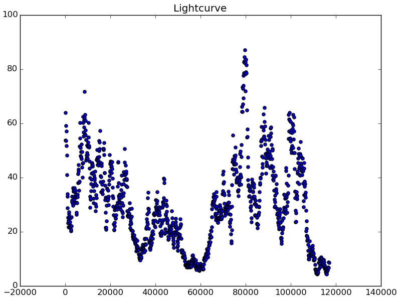
# estimate underlying variance od data light curve
datalc.STD_Estimate()


# simulate artificial light curve with Emmanoulopoulos method, using the PSD and PDF of the data
delc = datalc..Simulate_DE_Lightcurve() # defaults to bending PL and mix of gamma and lognormal dist.

# simulate artificial light curve with Timmer & Koenig method
tklc = Simulate_TK_Lightcurve(datalc,BendingPL, (A,v_bend,a_low,a_high,c),
                                RedNoiseL,aliasTbin,RandomSeed)

# simulate artificial light curve with Emmanoulopoulos method, scipy distribution
delc2 = Simulate_DE_Lightcurve(datalc,BendingPL, (A,v_bend,a_low,a_high,c),
                                ([st.gamma,st.lognorm],[[kappa,0, theta],\
                                    [lnsig,0, np.exp(lnmu)]],[weight,1-weight]))

# simulate artificial light curve with Emmanoulopoulos method, custom distribution
delc3 = Simulate_DE_Lightcurve(datalc,BendingPL, (A,v_bend,a_low,a_high,c),
                                ([[Gamma,LogNormal],[[kappa, theta],\
                                  [lnmu, lnsig]],[weight,1-weight]]),MixtureDist)

# plot lightcurves and their PSDs ands PDFs for comparison
Comparison_Plots([datalc,tklc,delc])
![alt tag] (https://raw.githubusercontent.com/samconnolly/DELightcurveSimulation/master/ComparisonPlots.png)
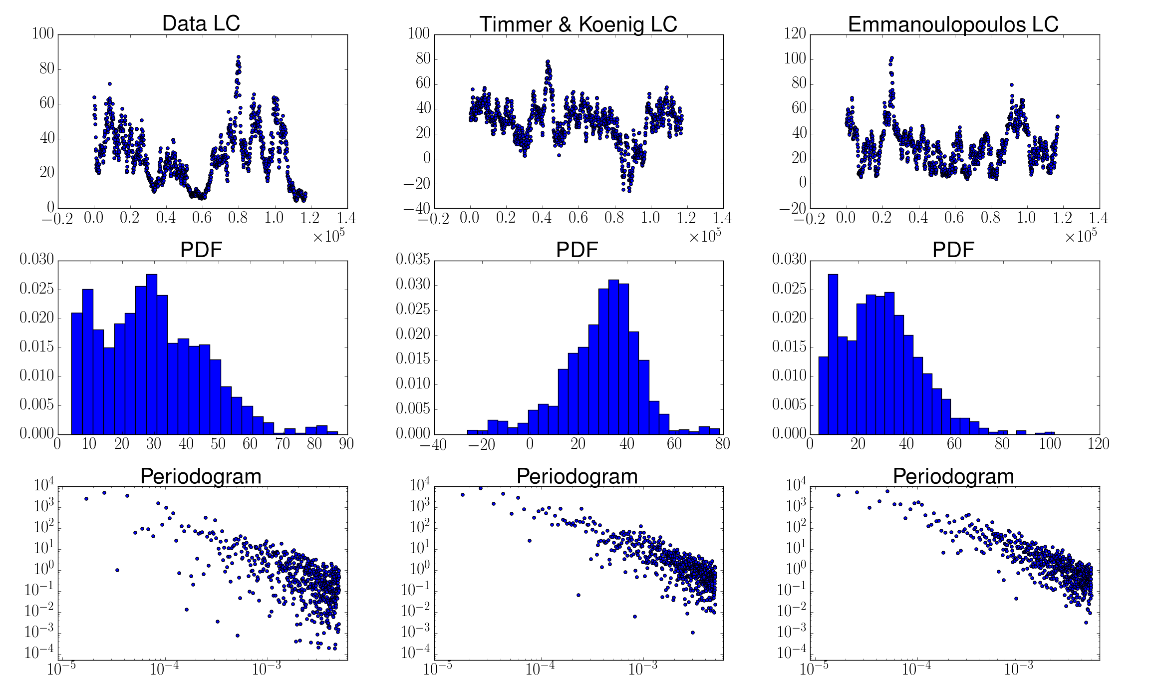
# Save lightcurve and Periodogram as text files
delc.Save_Lightcurve('lightcurve.dat')
delc.Save_Periodogram('periodogram.dat')