Tools Overview

| Option name | Description |
|---|---|
| Project | Manage, save, and load projects, including associated data and settings. |
| Export | Save various types of data generated within the software for external use. |
| Import | Bring external data into the software for processing and analysis. |
| Edit | Modify parameters, settings, and data within the current project. |
| Inverse tools | This section contains a variety of algorithms and methods that apply the lead field matrix to estimate the sources of neural activity within the brain based on measured electric or magnetic field data. These tools help identify specific brain regions responsible for a given pattern of neural activity. |
| Forward tools | This section focuses on creating the lead field matrix. These tools are applied before the inverse tools and are used for simulating and visualizing the electric or magnetic field patterns generated by a given set of neural sources. These tools help to understand how different source configurations affect the measured field patterns and can be useful for generating synthetic data for testing and validation purposes. |
| Multi-tools | The Multi-tools section contains various utilities that encompass multiple different tools or sets of tools. These tools can assist users in tasks such as working with 3D models, mesh data, and other types of information relevant to the simulation and analysis of brain activity. |
| Settings | Customize software preferences, configurations, and display options. |
| Window | Organize and navigate the software's multiple windows and views |
| Option name | Description |
|---|---|
| Volume data | The 3D volumetric representation of the head model, including information about the tissue types and their properties. |
| Segmentation data | The information about the segmented compartments or tissues within the head model, such as the brain, skull, and skin. This data includes the boundaries between different tissues, which can be used for mesh generation and calculations. |
| Lead field | The matrix that represents the relationship between the electric potential at the sensor locations (electrodes) and the source activity within the brain. |
| Source space | The 3D grid or mesh representing the possible locations of neural activity within the brain. This grid is used as the basis for estimating the neural activity from the measured electric potentials at the sensors. |
| Sensors | The information about the sensors or electrodes, including their positions, orientations, and other properties. |
| Reconstruction | Estimation of various neural activity distributions within the brain (e.g., electrical fields, blood flow) based on measured sensor data and lead field matrix. Reconstruction data can be visualized and analyzed to understand the underlying neural activity across different time frames. |
| FEM mesh | The finite element method (FEM) mesh representing the model's geometry and tissue properties |
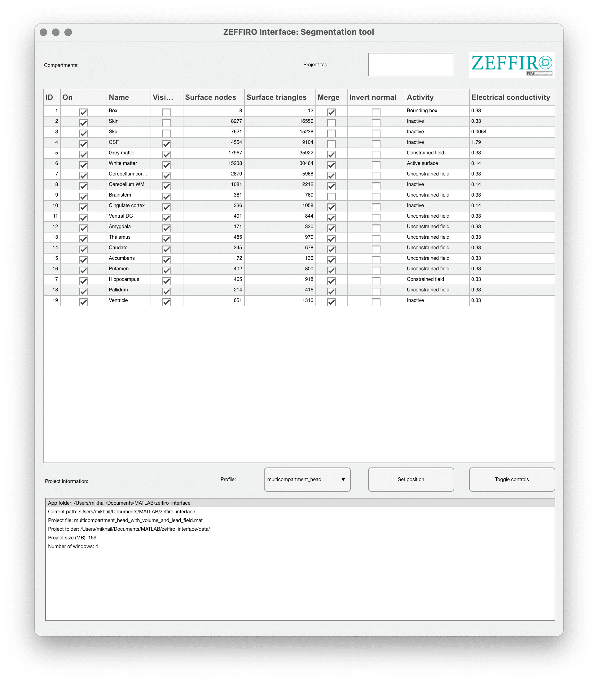
The main table of this window allow to control different compartments of the project. It may include more parameters than just Electrical conductivity by changing the profile (Advanced usage).
| Option name | Description |
|---|---|
| On | This checkbox indicates whether the compartment is active or not. An active compartment will be included in the calculations and simulations, while an inactive one will be ignored. |
| Name | Label for the compartment, which helps identify the specific region within the 3D model. |
| Visible | This checkbox determines whether the compartment is visible in the 3D view. |
| Surface nodes | Number of mesh grid nodes of the compartment. |
| Surface triangles | Number of triangular faces that make up the surface of the compartment. |
| Merge | This option allows you to combine two or more compartments into a single one. Merging can be useful for simplifying the model or combining structures that have similar properties. This option is used only during import. |
| Invert normal | This option is used to reverse the direction of the surface normals for the compartment. |
| Activity | Defines the role of the compartment in the model, including: - Bounding box: The compartment represents the outer boundary of the model. - Inactive: The compartment is not involved in the calculations. - Constrained field: The compartment is involved in the calculations but has some constraints applied. - Unconstrained field: The compartment is involved in the calculations without any constraints. - Active surface: The compartment represents an active surface, such as an electrode or a stimulating area. |
| Electrical conductivity | The electrical conductivity of the compartment or tissue, given in Siemens per meter (S/m). This value is used in the calculations to model the electrical properties of the tissue. |
This wiki page describes how to generate FEM mesh using ZI: Finite Element Mesh generation
This paper provides mathematical details about the mesh generation process: https://arxiv.org/abs/2203.10000
| Option name | Description |
|---|---|
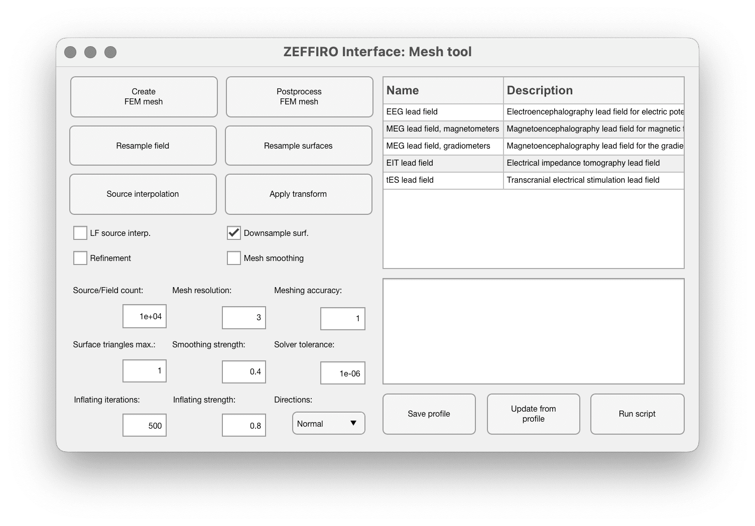
| Create FEM mesh | This option is used to generate a new FEM mesh based on the 3D model and segmentation data. Most important option |
| Postprocess FEM mesh | This function smooths the surfaces and optimizes the mesh structure, improving its quality and computational efficiency. It can be run after the mesh has been created to optimize it further. |
| Resample field and resample surfaces | These options allow users to control the number of sources in the FEM mesh and adjust the resolution of the surfaces. |
| Source interpolation | This function is run after creating a lead field, fixing the source positions in the reconstructed or simulated field. Second most important option |
| Apply transform | This button applies a transformation set in the segmentation tool, allowing users to modify the mesh based on various parameters. |
| Inflation | Creates an inflated surface representation of the brain's cortex. It expands the brain's cortical surface, reducing the complexity of the folding patterns (gyri and sulci). Note: Inflating in ZI works with the 3D mesh (tetrahedral) whereas recon-all inflation works with 2D surfaces. |
| Smoothing | It is used to apply a smoothing operation to the finite element mesh of the brain model |
| FL source interp. | Enables automatic source interpolation after running the mesh generation script. This allows to change the source space on the fly and reinterpret or resample the surfaces and fields separately |
| Downsample surf. | Better to leave it on. By enabling this checkbox, the ratio of surface triangles to mesh resolution is maintained, ensuring that the surface is appropriate for visualization. It's essential to note that the surface resolution is only used as a reference for plotting and does not directly impact the FEM mesh. |
| Refinement | This option turns on the refinement of the existing FEM mesh, increasing the resolution of reconstruction. The parameters of refinement are specified in Settings → Forward and Inverse processing options |
| Mesh smoothing | Enables the smoothing for the FEM mesh. For controlling the smoothing paramters see Settings → Forward and Inverse processing options, and find "Mesh smoothing and optimization" section. Smoothing is done by applying a Laplacian smoothing algorithm to the mesh. |
| Mesh resolution | The edges length in the initial FEM mesh (before refinement). Specified in millimeters. Start with value 3mm and refine the important brain regions, increasing their accuracy, so the FEM Mesh edge lengths will be reduced during that process. |
| Meshing accuracy | Better to set this value to 1 and not to change. |
| Surface triangles max | Specifies the maximum number of surface triangles relative to the targeted volumetric resolution. This value determines how much the surface mesh is upsampled or downsampled compared to the volumetric mesh resolution. This is a relative value (0.5 means downsample by factor 2, 2 means upsample by factor 2) |
| Inflating iterations | Controls the inflation for the surfaces, so this config doesn't impact the FEM Mesh itself, but changes the surfaces visualization. |
| Smoothing strength | The amount of inflation |
| Solver tolerance | |
| Inflating iterations | |
| Inflating strength |
Moreover, you can have even more control over the mesh refinement process by opening the Settings → Forward and Inverse processing options
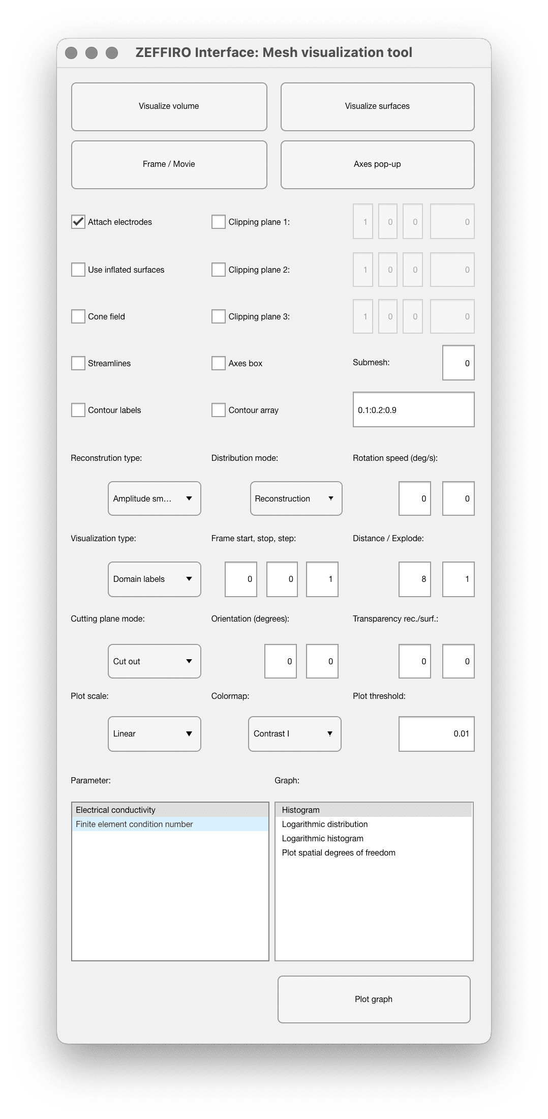
This tool focuses on visualizing the 3D mesh representation of the head model generated from the segmentation process. It allows manipulate various visualization parameters, such as clipping planes, orientations, and locations, to examine the model from different perspectives. Users can also toggle between visualizing volume and surfaces, making it easier to understand the head model's structure and properties.
There’s an additional set of configs, such as sensor point size, contour line width etc that could be found in Settings → Graphics processing options
Inflated surface: An inflated surface is a smoothed and expanded representation of the brain's cortical surface, which resembles a balloon-like shape. This representation is useful for visualizing and analyzing data across the entire brain surface without the complexities introduced by the intricate folding patterns of the cortex. By inflating the surface, researchers can more easily see and study the brain regions that would otherwise be hidden within the folds.
Folded surface: The folded surface represents the brain's cortex in its natural, convoluted state, with all its gyri (ridges) and sulci (grooves). While this representation is more anatomically accurate, it can be challenging to visualize and analyze data on the folded surface due to the complex geometry.
Some of these configurations could be further manipulated on the figure tool, but won't persist after closing the window.
| Option name | Description |
|---|---|
| Visualize Volume Button | Displays the volumetric data in the Figure tool window. This visualization includes the internal structure of the brain, such as different brain regions, and the distribution of the electric field within the volume of the brain tissue. |
| Visualize Surfaces Button | Displays the surface data of the 3D mesh. This includes the outer surfaces of the brain, such as the scalp, skull, and cortex, as well as the positions of the electrodes. This visualization provides a clear view of the brain's external features and how the electrodes are placed on the brain's surface. |
| Axes Pop-up Button | opens a separate window that displays the current axes of the 3D mesh visualization. This can be helpful to get a clear reference of the coordinate system while working with the mesh data and making adjustments to the visualization. |
| Clipping Plane Controls | Allow to customize the view by cutting away parts of the mesh to reveal the internal structure. |
| Attach Electrodes checkbox | used to visually fix the electrodes on the scalp or the nearest reference point in the mesh. This is necessary once the electrodes have been set in their final positions, to ensure that the volumetric model accurately represents the electrodes on the surface of the mesh. By checking this box, the electrodes are made to appear as if they are placed on the surface of the scalp, even if they deviate a little from their actual positions. This checkbox primarily affects the visualization of the electrodes, without significantly altering their actual locations. |
| Use inflated surfaces checkbox | Allows to switch between the inflated and folded surface representations |
| Reconstruction type | |
| Distribution mode | This config is applicable only to volume visualization. Reconstruction: will visualize the head compartments using the corresponding colors. Parameter real: will visualize a real part of the complex/real parameter selected below ("Parameter" section) Parameter imaginary: will visualize an imaginary part of the complex parameter |
| Rotation speed (deg/s) | Specify rotation of the model between different frames. Applicable for dynamic (multi-frame) models |
| Visualization type | This parameter selects the type of visualization and should match the button which is clicked for visualization |
| Start, stop, step | Controls the multi-frame model visualization |
| Cutting plane mode | Defines the direction of cut of cutting planes |
| Orientation (degrees) | Controls the initial orientation of the model |
| Transparency rec/surf | Initial transparency of visualized surfaces |
| Plot scale | Color map scale for parameter visualization |
| Colormap | Colormap for parameter visualization |
| Plot Threshold | Sets the lower limit for the intensity plot distribution. Important when dealing with logarithmic intensity plots, as the dynamic range can be extensive, making it difficult to visualize the data without a threshold, since an entire volume intensity is non-zero. |
| Parameter | This section allows to specify the parameter for visualizing (using "Visualize" buttons above) or plotting on a graph using "Plot graph" button below |
| Graph | Allows to choose the type of graph to be plotted by clicking "plot graph" button |
| Plot graph button | Plots the value specified in "parameter" section on a graph specified in "graph" section. This function requires having FEM mesh generated for current model |
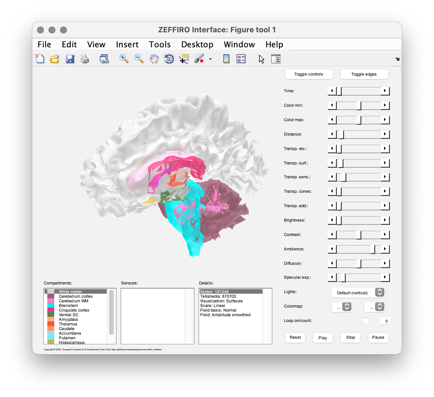
The Figure tool is designed for visualizing the head model and offers various sliders and controls that allow you to adjust the properties of the visualization in real-time. The "toggle controls" hides or shows the control panel, and "toggle edges" displays the finite element edges or polygons ( depending on the current visualization type).
| Option name | Description |
|---|---|
| Time | |
| Color min/max | |
| Distance | |
| Transp. rec | |
| Transp. surf | |
| Transp. sens. | |
| Transp. cones | |
| Transp. add | |
| Brightness | |
| Contrast | |
| Ambience | |
| Diffusion | |
| Specular exp. | |
| Lights | |
| Colormap | |
| Loop on/count |
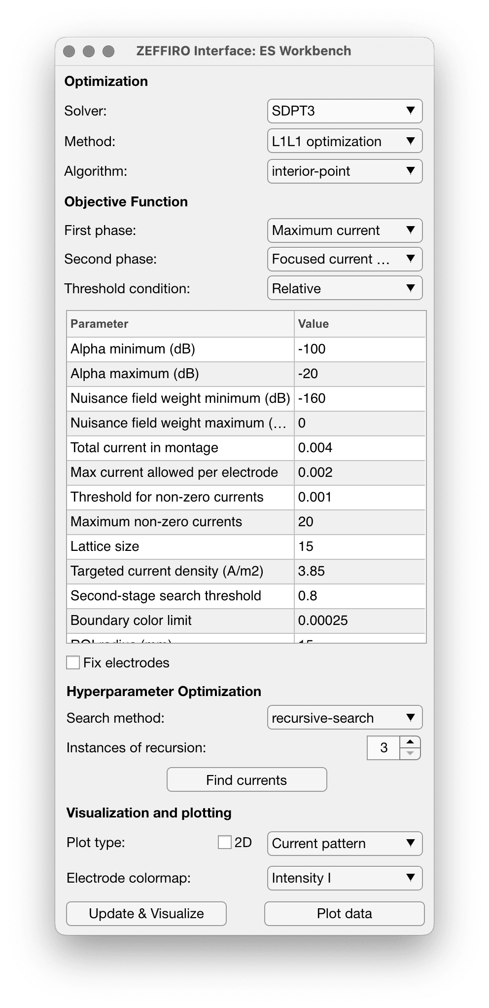
This tool allows to find optimal currents for brain simulation for a given set of electrodes using a set of computational methods.
| Option name | Description |
|---|---|
| Alpha (min/max) | The range of value of the alpha regularization parameter, controlling the balance between data fitting and regularization in the optimization algorithm. |
| Nuisance field weight (min/max) | aka ε (epsilon) - the weight assigned to the nuisance field in the optimization algorithm, controlling the balance between the focused and nuisance current densities. |
| Total current in montage | Sets the total current applied across all electrodes in the montage, ensuring safety and compliance with stimulation guidelines. See the https://www.sciencedirect.com/science/article/abs/pii/S1388245717302122 |
| Max current allowed per electrode | The maximum current that can be applied to each electrode in the montage. |
| Threshold for non-zero currents | The threshold below which a current is considered zero in the optimization algorithm. This parameter is used to promote sparsity in the solution. |
| Maximum non-zero currents | The maximum number of non-zero currents allowed in the optimization solution, controlling the greatest number of active electrodes. The optimization algorithm will select given number of electrodes with greatest magnitude. |
| Lattice size | The size of the lattice used in the optimization algorithm, affecting the granularity of the search space. |
| Target current density | The desired current density at the target location in the brain, used as an objective for the optimization algorithm. |
| Second-stage search threshold | The threshold used in the second-stage search of the optimization algorithm, determining which solutions from the first stage are further refined. |
| Boundary color limit | The limit for the color scale used to visualize the electrodes in the Figure tool. Does not impact the optimization |
| ROI radius (mm) | The radius of the region of interest (ROI) around the target location, defining the volume within which the optimization algorithm tries to maximize the focused current density. |
| Solver tolerance | The tolerance for the solver used in the optimization algorithm, determining the accuracy and convergence of the solution. |
| Display | A parameter controlling the display of intermediate results and progress during the optimization process, useful for monitoring the algorithm's performance. |
| Maximum number of iterations | The maximum number of iterations allowed for the optimization algorithm, controlling the computational time and resources spent on the optimization process. |
| Solver | Allows to specify the engine for the computations. All besides MOSEK and Gurobi are installed along with ZI. Different engines can have different performance. |
| Method | |
| Algorithm | |
| First phase objective function | |
| Second phase objective function | |
| Threshold condition | |
| Fix electrodes | |
| 2D plot type |
| Option name | Description |
|---|---|
| Residual | The difference between the observed data and the predicted data from the optimization algorithm. A lower residual indicates a better fit. |
| Max current | The maximum amount of electrical current being delivered to a specific electrode. |
| Sparsity (2-norm/1-norm) ratio | A measure of how sparse or localized the current distribution is. A higher ratio indicates a more localized current distribution |
| Focused current density | The amount of current density at the target region (ROI), indicating the strength of the stimulation at that specific area. |
| Nuisance current density | The amount of current density in non-targeted areas of the brain, which can potentially cause unwanted side effects or stimulation of other brain regions. |
| Angle error | The difference in angle between the desired and actual current vector direction. A smaller angle error indicates a better alignment between the actual and desired stimulation direction. Measured in degrees. |
| Relative magnitude difference | The difference in magnitude between the desired and actual current magnitudes. Minimizing this difference ensures that the electric field is closer to the desired strength. |
| RDM (Relative difference measure) | Difference between two unit vectors pointing at target and achieved between electric field distributions, ranges from 0.0 to 2.0 (or 200%), the lower the better |
| Field ratio | The ratio of the focused current density to the nuisance current density, indicating how effectively the current is focused on the target region compared to non-target regions. Computed as Focused/Nuisance |
| NNZ | The number of non-zero elements in the solution, indicating the sparsity or complexity of the electrode configuration. |
| Total dose | The total amount of electrical current delivered to the brain during the stimulation session. |
| Run time | The time it takes for the optimization algorithm to compute the solution. |
| Alpha | A regularization parameter α that controls the balance between data fitting and solution sparsity in the optimization algorithm. |
| Beta | ??? |
| Optimizer flag value | A value indicating the status of the optimization algorithm, such as whether it has converged to a solution or encountered an error. 1 means “all ok” |
| lattice run time(s) | The time it takes for the optimization algorithm to perform a specific operation or computation, such as searching through a lattice of candidate solutions. |
In ZI, a mesh imported from FreeSurfer can be equipped with a parcellation. A parcellation can be imported using the Parcellation tool. A colortable and points (labels) produced by FreeSurfer can be imported via Colortable and Points buttons. Colortable refers to a .MAT file containing the vertices, label, and colortable variables generated by FreeSurfer's Matlab interface function read_annotation. The points refer to an .ASC file produced by FreeSurfer's mri_mergelabels function. However, also other parcellation types than those of FreeSurfer can be imported. Several parcellation segments (for the left and right hemisphere) can be merged. The segmentation including all of its active subcompartments can be included in the parcellation by pressing the Segmentation button.
After importing the segmentation, one can select some or all of the regions within the parcellation list (Figure 6) and interpolate them into the source basis of the lead field by pressing Interpolate. The intepolated regions can be visualized on the brain by selecting the option Parcellation for both the colormap (in Options) and the visualization type (in Mesh tool). To visualize a parcellation or to restrict an inverse estimate to the selected regions the status of the parcellation must be Active.
Time series will analyze any inverse estimate in the selected regions (a single one or a sequence) with respect to the selected reconstruction type. The results, e.g., correlation, can be plotted by pressing Plot. In the Options menu, one can select whether a point-wise value or a quantile taken over a region is considered.

Figure: A parcellation interpolated on a 1 mm brain model and visualized with the
Parcellation option (for colormap and visualization type).

Figure:
Time series correlation calculated for the selected brain regions after reconstructing the brain activity.