These are the code examples written by François Chollet, author of Keras. Base image by yours truly.

NST uses deep neural networks and allows you to transfer the style of 1 (style) image onto another (content) image. Pixel values are used as weights and biases to train the image to generate instead of making and training a model.
It was first published in the paper "A Neural Algorithm of Artistic Style" proposed by Leon A. Gatys, Alexander S. Ecker and Matthias Bethge in 2015.
Although it isn't "state of the art" and already used in Photoshop (neural filters) and mobile apps such as Copista, it is still interesting to see how it works and what can be created by changing parameters and hyper-parameters.
The key finding of the paper is that the representations of content and style in the Convolutional neural network are separable.
The class of Deep Neural Networks that are most powerful in image processing tasks are called Convolutional Neural Networks (CNN or ConvNet).
The name convolutional comes from a function which maps a tuple of sequences into a sequence of tuples. It is a linear operation and convolutional networks are simply neural networks that use convolution in place of general matrix multiplication in at least one of their layers.
CNN = small computational units that process visual information hierarchically feed-forward. These networks care more about the higher layers such as shape and content (the more technical features).
Each layer of units = a collection of image filters, each of which extracts a certain feature from the input image.
Thus, the output of a given layer consists of so-called feature maps: differently filtered versions of the input image.
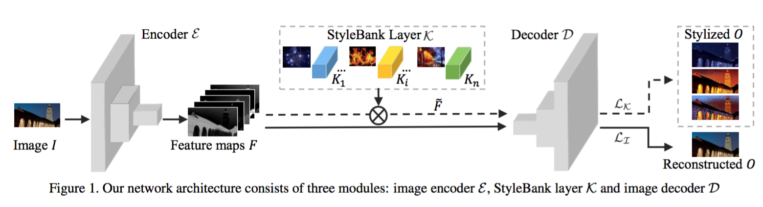
So a feature map is the output of 1 filter applied to the previous layer. A given filter is drawn across the entire previous layer, moved 1 pixel at a time. Each position results in an activation of the neuron and the output is collected in the feature map.
The name stems from the authors → Visual Geometry Group at Oxford. The results presented in the main text were generated on the basis of the VGG-Network, a CNN that rivals human performance on a common visual object recognition benchmark task.
In the code example below VGG19 is used. This CNN is 19 layers deep, and it classifies images. You can load a pre-trained version of the network trained on more than a million images from the ImageNet database. The pre-trained network can classify images into 1000 object categories, such as keyboard, mouse, pencil, and many animals. As a result, the network has learned rich feature representations for a wide range of images. The network has an image input size of 224-by-224 by default.
For the original contents. The programming language is Python and for (free) GPU we can use Google Colab and Kaggle Notebook.
Table of contents:
- Pre-processing utilities
- De-processing utilities
- Compute the style transfer loss
- Gram matrix
- style_loss function
- content_loss function
- total_variation_loss function
- Feature extraction model that retrieves intermediate activations of VGG19.
- Finally, here's the code that computes the style transfer loss.
- Add a tf.function decorator to loss & gradient computation.
- The training loop
- References
- Tools
Util function to open, resize and format pictures into appropriate tensors (multidimensional arrays).
def preprocess_image(image_path):
    img = keras.preprocessing.image.load_img(
        image_path, target_size=(img_nrows, img_ncols)
    )
    img = keras.preprocessing.image.img_to_array(img)
    img = np.expand_dims(img, axis=0)
    img = vgg19.preprocess_input(img)
return tf.convert_to_tensor(img)Util function to convert a tensor into a valid image.
def deprocess_image(x):
    x = x.reshape((img_nrows, img_ncols, 3))
Remove zero-centre by mean pixel.
Zero-centring = shifting the values of the distribution to set the mean = 0. Removing zero-centre by mean pixel is a common practise to improve accuracy.
Mathematically this can be done by calculating the mean in your images and subtracting each image item with that mean. The mean and standard deviation required to standardize pixel values can be calculated from the pixel values in each image only (sample-wise) or across the entire training dataset (feature-wise).
NumPy allows us to specify the dimensions over which a statistic like the mean, min, and max are calculated via the “axis” argument. Source.
VGG19 is trained with each channel normalised by mean = [103.939, 116.779, 123.68]. These are the constants to use when working with this network.
    x[:, :, 0] += 103.939
    x[:, :, 1] += 116.779
    x[:, :, 2] += 123.68
'BGR'->'RGB'
R(ed)G(reen)B(lue) is the colour model for the sensing, representation, and display of images. These are the primary colours of light (although light itself is an electromagnetic wave and colourless) and maximise the range perceived by the eyes and brain. Because we are working with screens that emit light instead of pigments, we use RGB.
The model formats the input image as batch size, channels, height and width as a NumPy-array in the form of BGR. VGG19 was trained using Caffe which uses OpenCV to load images and has BGR by default, therefore 'BGR'→'RGB' or x = x[:, :, ::-1] because this is how you reverse it.
Clip the interval edges to 0 and 255 otherwise we may pick values between −∞ and +∞. Red, green and blue use 8 bits each, and they have integer values ranging from 0 to 255. 256³ = 16777216 possible colours. The data type = uint8 = Unsigned Integers of 8 bits (there are only 8 bits of information). Unsigned integers are integers without a "-" or "+" assigned to them. They are always non-negative (0 or positive) and we use them if we know that the outcome will always be non-negative.
    x = x[:, :, ::-1]
    x = np.clip(x, 0, 255).astype("uint8")
return xThe loss/cost is the difference between the original and the generated image. We can calculate this in different ways (MSE, Euclidean distance, etc.). By minimising the differences of the images, we are able to transfer style.
As commented in the code by Mr. Chollet.
The "style loss" is designed to maintain the style of the reference image in the generated image. It is based on the gram matrices (which capture style) of feature maps from the style reference image and from the generated image. First, we need to define 4 utility functions:
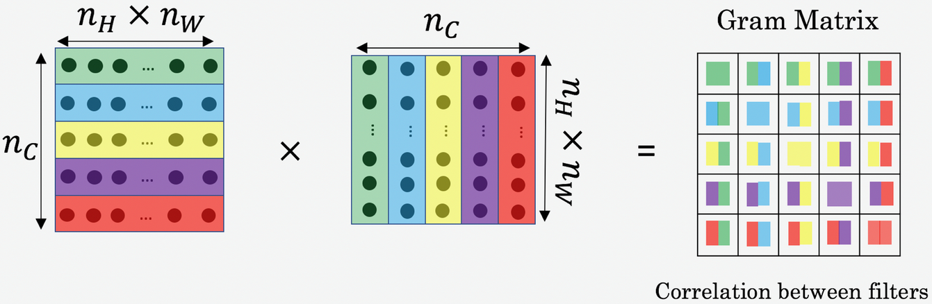
1. Gram matrix: If we want to extract the style of an image, we need to compute the style-loss/cost. To do this we make use of the Gram matrix because it is the correlations between feature maps.
The Gram matrix is the multiplication (the dot product) of a matrix with its transpose.
Transpose: In linear algebra, the transpose of a matrix is an operator which flips a matrix over its diagonal; that is, it switches the row and column indices of the matrix M by producing another matrix, often denoted by Mᵀ.
So we multiply matrix M with its transpose and the values will tell you the similarities between the feature maps or channels.
We do height x width to create a 1 dimension = the number of neurons and activation functions per channel. Then we are multiplying the values of channel 1 with the values of channel 2 to find the similarities between them.
Why does the Gram matrix represent artistic style? This is explained in the paper Demystifying Neural Style Transfer proposed by Yanghao Li, Naiyan Wang, Jiaying Liu and Xiaodi Hou in 2017.
We theoretically prove that matching the Gram matrices of the neural activations can be seen as minimising a specific Maximum Mean Discrepancy (MMD) [Gretton et Aal., 2012a]. This reveals that neural style transfer is intrinsically a process of distribution alignment of the neural activations between images.
When we are minimising the style loss, we are matching the distribution of features between two images. The gram matrix able to capture that distribution alignment of those feature maps in a given layer.
def gram_matrix(x):
    x = tf.transpose(x, (2, 0, 1))
    features = tf.reshape(x, (tf.shape(x)[0], -1))
    gram = tf.matmul(features, tf.transpose(features))
    return gram
For the finite-dimensional real vector in R^n with the usual Euclidean dot product, the Gram matrix is simply G = V^T x V, where V is a matrix whose columns are the vectors V(k).
Why the dot product? The dot product takes two equal-length sequences of numbers and returns a single number → a · b = |a| × |b| × cos(θ) or we can do → a · b = ax × bx + ay × by
Let’s take 2 flattened vectors representing features of the input space. The dot product gives us information about the relation between them. It shows us how similar they are.
In other words, the closer the 2 vectors are, the smaller the angle and the more similar they are. The smaller the value of the angle, the bigger the cosine (because of trigonometry...), so —>
- The lesser the product = the more different the learned features are.
- The greater the product = the more correlated the features are.
2. The style_loss function: Which keeps the generated image close to the local textures of the style reference image.
We take the Gram matrix of the activations at each layer in the network for both images. For a single image, the Gram matrix of its activations at a layer is given by:
= the dot product between the vectorised feature map
and
in layer
.
= where
is the representation of the generated image and where
is the vectorised feature map in layer
. It is the activation for the
-th feature map at layer
.
= where
is the representation of the generated image and where
is the vectorised feature map in layer
. It is the activation for the
-th feature map at layer
.
We can now define the style loss at a single layer as the Euclidean (L2) distance between the Gram matrices of the style and output images.
= the Euclidean (L2) distance between the Gram matrices of the style and output images.
= a layer with
distinct filters
has
feature maps each of size
.
= the height times the width of the feature map.
= the respective style representation in layer
of the generated image
.
= the respective style representations in layer
of the original
.
The last step is to compute the total style loss as a weighted sum of the style loss at each layer.
= weighting factors of the contribution of each layer to the total loss.
def style_loss(style, combination):
    S = gram_matrix(style)
    C = gram_matrix(combination)
    channels = 3
    size = img_nrows * img_ncols
    return tf.reduce_sum(tf.square(S - C)) / (4.0 * (channels ** 2) * (size ** 2))
3. The content_loss function: Which keeps the high-level representation of the generated image close to that of the base image. An auxiliary loss function designed to maintain the "content" of the base image in the generated image.
So let p⃗ and x⃗ be the original image and the image that is generated and and
their respective feature representation in layer
. We then define the squared-error loss between the two feature representations.
def content_loss(base, combination):
    return tf.reduce_sum(tf.square(combination - base))
4. The total_variation_loss function: This is a regularisation loss to improve the smoothness of the generated image by keeping it locally-coherent and ensuring spatial continuity. This wasn’t used in the original paper. It was later added because optimisation to reduce only the style and content losses led to highly pixelated and noisy outputs. We are basically shifting pixel values. It is defined in the following function.
def total_variation_loss(x): a = K.square( x[:, :img_height - 1, :img_width - 1, :] - x[:, 1:, :img_width - 1, :]) b = K.square( x[:, :img_height - 1, :img_width - 1, :] - x[:, :img_height - 1, 1:, :])
return K.sum(K.pow(a + b, 1.25))
or in this case:
def total_variation_loss(x):
    a = tf.square(
        x[:, : img_nrows - 1, : img_ncols - 1, :] - x[:, 1:, : img_ncols - 1, :]
    )
    b = tf.square(
        x[:, : img_nrows - 1, : img_ncols - 1, :] - x[:, : img_nrows - 1, 1:, :]
    )
return tf.reduce_sum(tf.pow(a + b, 1.25))#Build a VGG19 model loaded with pre-trained ImageNet weights
model = vgg19.VGG19(weights="imagenet", include_top=False)
# Get the symbolic outputs of each "key" layer (we gave them unique names).
outputs_dict = dict([(layer.name, layer.output) for layer in model.layers])
# Set up a model that returns the activation values for every layer in
# VGG19 (as a dict).
feature_extractor = keras.Model(inputs=model.inputs, outputs=outputs_dict)# List of layers to use for the style loss.
style_layer_names = [
"block1_conv1",
"block2_conv1",
"block3_conv1",
"block4_conv1",
"block5_conv1",
]
# The layer to use for the content loss.
content_layer_name = "block5_conv2"
def compute_loss(combination_image, base_image, style_reference_image):
input_tensor = tf.concat(
[base_image, style_reference_image, combination_image], axis=0
)
features = feature_extractor(input_tensor)
# Initialize the loss
loss = tf.zeros(shape=())
# Add content loss
layer_features = features[content_layer_name]
base_image_features = layer_features[0, :, :, :]
combination_features = layer_features[2, :, :, :]
loss = loss + content_weight * content_loss(
base_image_features, combination_features
)
# Add style loss
for layer_name in style_layer_names:
layer_features = features[layer_name]
style_reference_features = layer_features[1, :, :, :]
combination_features = layer_features[2, :, :, :]
sl = style_loss(style_reference_features, combination_features)
loss += (style_weight / len(style_layer_names)) * sl
# Add total variation loss
loss += total_variation_weight * total_variation_loss(combination_image)
return lossTo compile it and thus make it fast. A decorator enables us to add functionalities to objects without changing the structure. TensorFlow provides the tf.GradientTape API for automatic differentiation; that is, computing the gradient of a computation with respect to some inputs, usually tf.Variables.
@tf.function
def compute_loss_and_grads(combination_image, base_image, style_reference_image):
    with tf.GradientTape() as tape:
        loss = compute_loss(combination_image, base_image, style_reference_image)
    grads = tape.gradient(loss, combination_image)
return loss, gradsRepeatedly run vanilla gradient descent steps to minimise the loss and save the resulting image every 100 iterations. We decay the learning rate by 0.96 every 100 steps.
Here, the optimisation algorithm is Stochastic Gradient Descent (SGD). Stochastic = having a random probability distribution or pattern that may be analysed statistically but may not be predicted precisely (oxford-languages).
It goes through the entire data set and replaces the gradient with an estimate thereof. The estimates are calculated from a randomly selected subset of that data. This optimiser has been in use since the sixties (of the last century). We are optimising pixel values instead of the parameters.
We can, of course, experiment with different optimisers to see which one gives the most desirable outcome.
optimizer = keras.optimizers.SGD(
    keras.optimizers.schedules.ExponentialDecay(
        initial_learning_rate=100.0, decay_steps=100, decay_rate=0.96
    )
)

base_image = preprocess_image(base_image_path)
style_reference_image = preprocess_image(style_reference_image_path)
combination_image = tf.Variable(preprocess_image(base_image_path))

iterations = 4000
for i in range(1, iterations + 1):
    loss, grads = compute_loss_and_grads(
        combination_image, base_image, style_reference_image
    )
    optimizer.apply_gradients([(grads, combination_image)])
    if i % 100 == 0:
        print("Iteration %d: loss=%.2f" % (i, loss))
        img = deprocess_image(combination_image.numpy())
        fname = result_prefix + "_at_iteration_%d.png" % i
keras.preprocessing.image.save_img(fname, img)Neural Style Transfer:
-
A Neural Algorithm of Artistic Style by Leon A. Gatys, Alexander S. Ecker and Matthias Bethge
-
Demystifying Neural Style Transfer by Yanghao Li, Naiyan Wang, Jiaying Liu and Xiaodi Hou
Convolutional Neural Networks:
-
A Comprehensive Guide to Convolutional Neural Networks — the ELI5 way
-
How Do Convolutional Layers Work in Deep Learning Neural Networks?
VGG19:
Tensors:
-
GPU: Google Colab and Kaggle Notebook
-
Equation editor: CodeCogs