The goals / steps of this project are the following:
- Compute the camera calibration matrix and distortion coefficients given a set of chessboard images.
- Apply a distortion correction to raw images.
- Use color transforms, gradients, etc., to create a thresholded binary image.
- Apply a perspective transform to rectify binary image ("birds-eye view").
- Detect lane pixels and fit to find the lane boundary.
- Determine the curvature of the lane and vehicle position with respect to center.
- Warp the detected lane boundaries back onto the original image.
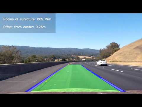
- Output visual display of the lane boundaries and numerical estimation of lane curvature and vehicle position.
The code for this step is contained in the "Camera Calibration" code cell of the IPython notebook Advanced Lane Detection.ipynb
I start by preparing "object points", which will be the (x, y, z) coordinates of the chessboard corners in the world. Here I am assuming the chessboard is fixed on the (x, y) plane at z=0, such that the object points are the same for each calibration image. Thus, objp is just a replicated array of coordinates, and objpoints will be appended with a copy of it every time I successfully detect all chessboard corners in a test image. imgpoints will be appended with the (x, y) pixel position of each of the corners in the image plane with each successful chessboard detection.
I then used the output objpoints and imgpoints to compute the camera calibration and distortion coefficients using the cv2.calibrateCamera() function. I applied this distortion correction to the test image using the cv2.undistort() function and obtained this result:

After camera calibration, I used the distortion coefficients and camera matrix to undistort the road images. It is hard to notice the corrected distortion in the image below except on the extreme left and right:

Coming up with a good threshold for binarizing the image is a very crucial task because the whole pipeline depends on it.
The code for this step is contained in the "Image Binarization" code cell of the IPython notebook Advanced Lane Detection.ipynb
For detecting yellow lines, I used a threshold on V channel in the HSV color space. For white lines, equalizing the histrogram really helped. Lastly, I used a Sobel mask to detect the gradients of lines. I combined the output of all of the above thresholding methods to get the following output:

The code for my perspective transform includes a function called perpective(), which appears in "Perpective View" cell of the notebook. The perpective() function takes as inputs an image (img), as well as source (src) and destination (dst) points. I chose the following source and destination points:
src = np.float32([[w, h-15], [0, h-15], [546, 460], [732, 460]])
dst = np.float32([[w, h], [0, h], [0, 0], [w, 0]])
I verified that my perspective transform was working as expected by visualizing a test image and its warped counterpart.

When fitting polynomials to lane lines, there are 2 cases:
- New image - I use the
sliding_windows()function to find the peak locations of the histogram of the binary image, and then slide two windows towards the upper side of the image, deciding which pixels belong to the lane line. - In case of video processing, we can limit our search in the neighbourhood of previously detected lane lines. I do this using the method
approx_by_previous_fits()

The offset from the lane center can be computed assuming that the camera is fixed and mounted in the midpoint of the car roof. In this case, we can approximate the car's deviation from the lane center as the distance between the center of the image and the midpoint at the bottom of the image of the two lane-lines detected. This is done using the method compute_offset_from_center().
The radius of curvature can be computed using the coefficients of 2nd degree polynomial fitted to the lane lines. I did this in the method curvature_meter().
The whole pipeline produces the following image:
Other images can be found in the output_images directory.

One of the main issues that I see with the approaches in this project is the selection of parameters by hand for these specific road images. This clearly makes this approach hard to generalize. The pipeline is very fragile to image changes such as variations in brightness, contrast etc. as the thresholding parameters have been hardcoded and the whole pipeline depends heavily on the binarized image.