all-classification-templetes-for-ML

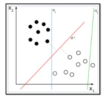
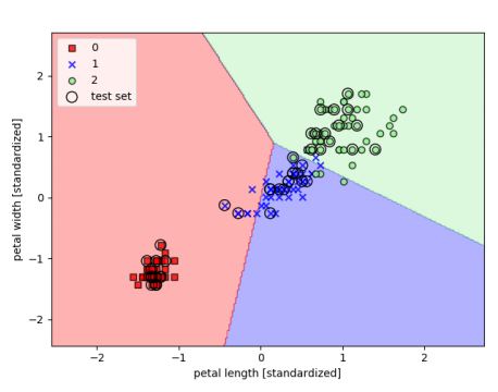
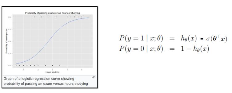
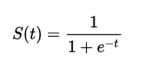
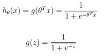
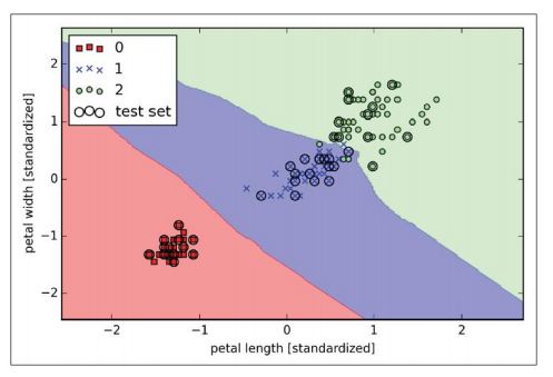
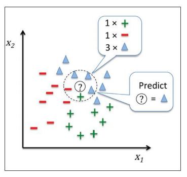
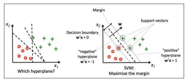
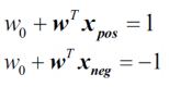
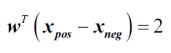
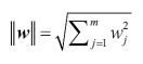
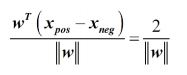
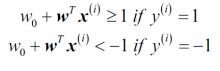
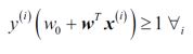
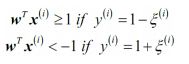
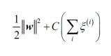
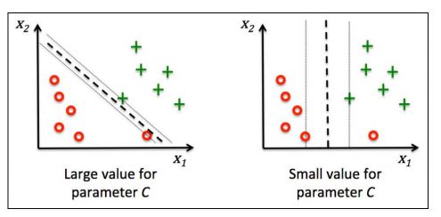
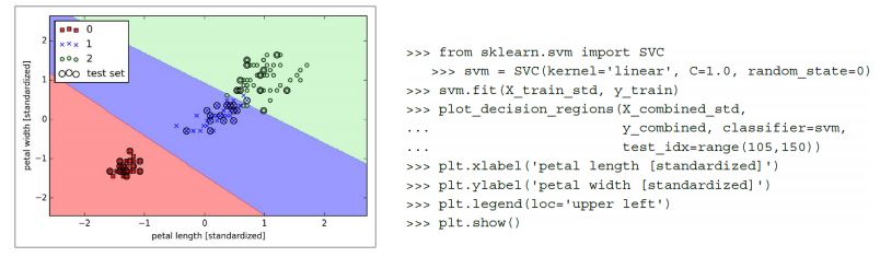
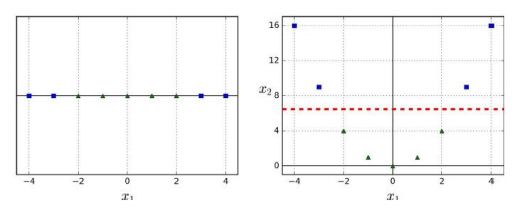
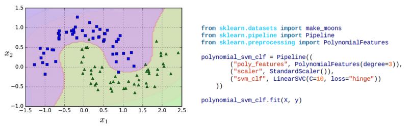
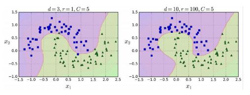
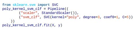
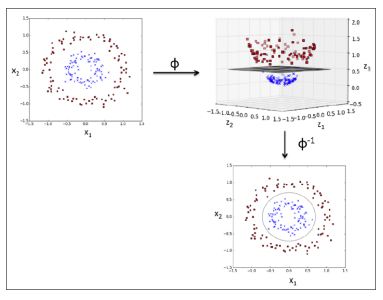
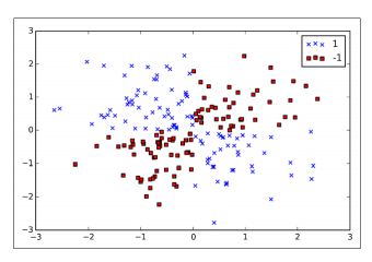
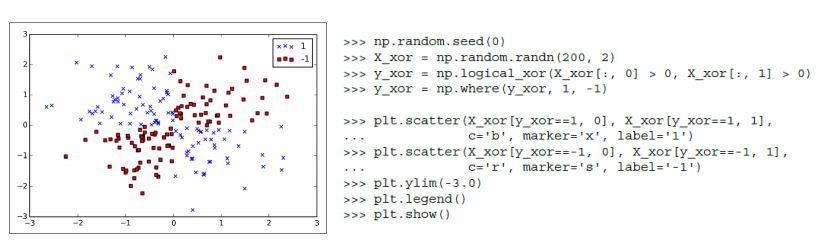
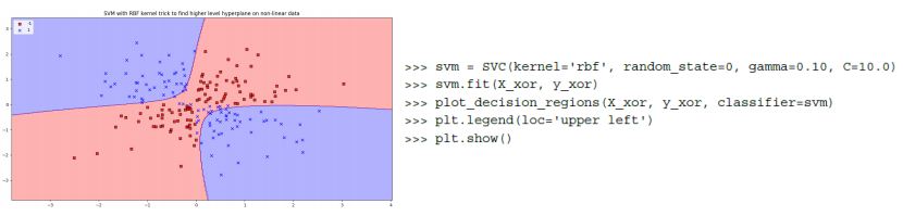
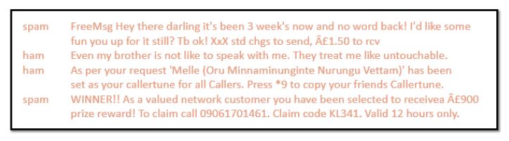
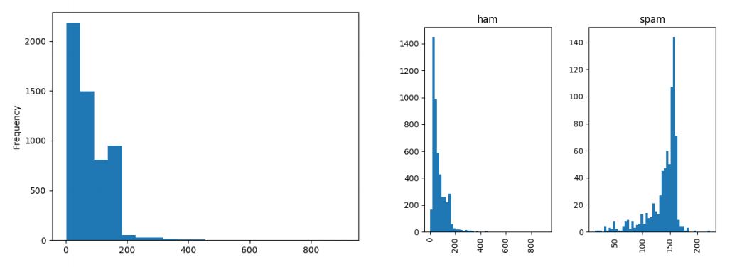
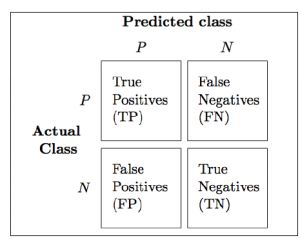
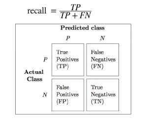
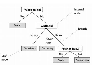
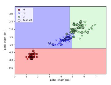
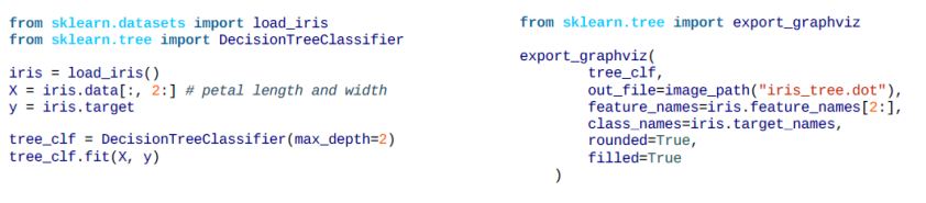
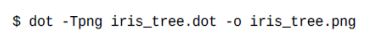
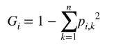
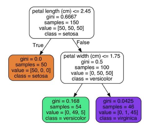
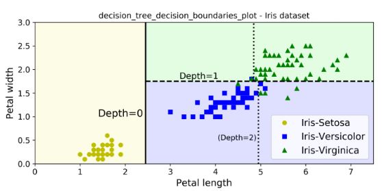
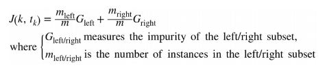
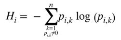
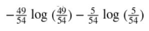
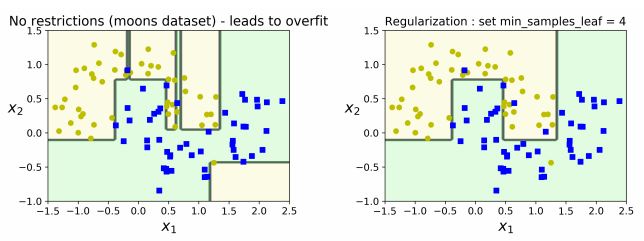
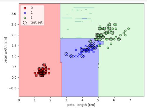
Classification - Machine Learning This is ‘Classification’ tutorial which is a part of the Machine Learning course offered by Simplilearn. We will learn Classification algorithms, types of classification algorithms, support vector machines(SVM), Naive Bayes, Decision Tree and Random Forest Classifier in this tutorial. Objectives Let us look at some of the objectives covered under this section of Machine Learning tutorial. Define Classification and list its algorithms Describe Logistic Regression and Sigmoid Probability Explain K-Nearest Neighbors and KNN classification Understand Support Vector Machines, Polynomial Kernel, and Kernel Trick Analyze Kernel Support Vector Machines with an example Implement the Naïve Bayes Classifier Demonstrate Decision Tree Classifier Describe Random Forest Classifier Classification: Meaning Classification is a type of supervised learning. It specifies the class to which data elements belong to and is best used when the output has finite and discrete values. It predicts a class for an input variable as well. There are 2 types of Classification: Binomial Multi-Class Classification: Use Cases Some of the key areas where classification cases are being used: To find whether an email received is a spam or ham To identify customer segments To find if a bank loan is granted To identify if a kid will pass or fail in an examination Classification: Example Social media sentiment analysis has two potential outcomes, positive or negative, as displayed by the chart given below. https://www.simplilearn.com/ice9/free_resources_article_thumb/classification-example-machine-learning.JPG This chart shows the classification of the Iris flower dataset into its three sub-species indicated by codes 0, 1, and 2. https://www.simplilearn.com/ice9/free_resources_article_thumb/iris-flower-dataset-graph.JPG The test set dots represent the assignment of new test data points to one class or the other based on the trained classifier model. Types of Classification Algorithms Let’s have a quick look into the types of Classification Algorithm below. Linear Models Logistic Regression Support Vector Machines Nonlinear models K-nearest Neighbors (KNN) Kernel Support Vector Machines (SVM) Naïve Bayes Decision Tree Classification Random Forest Classification Logistic Regression: Meaning Let us understand the Logistic Regression model below. This refers to a regression model that is used for classification. This method is widely used for binary classification problems. It can also be extended to multi-class classification problems. Here, the dependent variable is categorical: y ϵ {0, 1} A binary dependent variable can have only two values, like 0 or 1, win or lose, pass or fail, healthy or sick, etc In this case, you model the probability distribution of output y as 1 or 0. This is called the sigmoid probability (σ). If σ(θ Tx) > 0.5, set y = 1, else set y = 0 Unlike Linear Regression (and its Normal Equation solution), there is no closed form solution for finding optimal weights of Logistic Regression. Instead, you must solve this with maximum likelihood estimation (a probability model to detect the maximum likelihood of something happening). It can be used to calculate the probability of a given outcome in a binary model, like the probability of being classified as sick or passing an exam. https://www.simplilearn.com/ice9/free_resources_article_thumb/logistic-regression-example-graph.JPG Sigmoid Probability The probability in the logistic regression is often represented by the Sigmoid function (also called the logistic function or the S-curve): https://www.simplilearn.com/ice9/free_resources_article_thumb/sigmoid-function-machine-learning.JPG In this equation, t represents data values * the number of hours studied and S(t) represents the probability of passing the exam. Assume sigmoid function: https://www.simplilearn.com/ice9/free_resources_article_thumb/sigmoid-probability-machine-learning.JPG g(z) tends toward 1 as z -> infinity , and g(z) tends toward 0 as z -> infinity K-nearest Neighbors (KNN) K-nearest Neighbors algorithm is used to assign a data point to clusters based on similarity measurement. It uses a supervised method for classification. The steps to writing a k-means algorithm are as given below: https://www.simplilearn.com/ice9/free_resources_article_thumb/knn-distribution-graph-machine-learning.JPG Choose the number of k and a distance metric. (k = 5 is common) Find k-nearest neighbors of the sample that you want to classify Assign the class label by majority vote. KNN Classification A new input point is classified in the category such that it has the most number of neighbors from that category. For example: https://www.simplilearn.com/ice9/free_resources_article_thumb/knn-classification-machine-learning.JPG Classify a patient as high risk or low risk. Mark email as spam or ham. Keen on learning about Classification Algorithms in Machine Learning? Click here! Support Vector Machine (SVM) Let us understand Support Vector Machine (SVM) in detail below. SVMs are classification algorithms used to assign data to various classes. They involve detecting hyperplanes which segregate data into classes. SVMs are very versatile and are also capable of performing linear or nonlinear classification, regression, and outlier detection. Once ideal hyperplanes are discovered, new data points can be easily classified. https://www.simplilearn.com/ice9/free_resources_article_thumb/support-vector-machines-graph-machine-learning.JPG The optimization objective is to find “maximum margin hyperplane” that is farthest from the closest points in the two classes (these points are called support vectors). In the given figure, the middle line represents the hyperplane. SVM Example Let’s look at this image below and have an idea about SVM in general. Hyperplanes with larger margins have lower generalization error. The positive and negative hyperplanes are represented by: https://www.simplilearn.com/ice9/free_resources_article_thumb/positive-negative-hyperplanes-machine-learning.JPG Classification of any new input sample xtest : If w0 + wTxtest > 1, the sample xtest is said to be in the class toward the right of the positive hyperplane. If w0 + wTxtest < -1, the sample xtest is said to be in the class toward the left of the negative hyperplane. When you subtract the two equations, you get: https://www.simplilearn.com/ice9/free_resources_article_thumb/equation-subtraction-machine-learning.JPG Length of vector w is (L2 norm length): https://www.simplilearn.com/ice9/free_resources_article_thumb/length-of-vector-machine-learning.JPG You normalize with the length of w to arrive at: https://www.simplilearn.com/ice9/free_resources_article_thumb/normalize-equation-machine-learning.JPG SVM: Hard Margin Classification Given below are some points to understand Hard Margin Classification. The left side of equation SVM-1 given above can be interpreted as the distance between the positive (+ve) and negative (-ve) hyperplanes; in other words, it is the margin that can be maximized. Hence the objective of the function is to maximize with the constraint that the samples are classified correctly, which is represented as : https://www.simplilearn.com/ice9/free_resources_article_thumb/hard-margin-classification-machine-learning.JPG This means that you are minimizing ‖w‖. This also means that all positive samples are on one side of the positive hyperplane and all negative samples are on the other side of the negative hyperplane. This can be written concisely as : https://www.simplilearn.com/ice9/free_resources_article_thumb/hard-margin-classification-formula.JPG Minimizing ‖w‖ is the same as minimizing. This figure is better as it is differentiable even at w = 0. The approach listed above is called “hard margin linear SVM classifier.” SVM: Soft Margin Classification Given below are some points to understand Soft Margin Classification. To allow for linear constraints to be relaxed for nonlinearly separable data, a slack variable is introduced. (i) measures how much ith instance is allowed to violate the margin. The slack variable is simply added to the linear constraints. https://www.simplilearn.com/ice9/free_resources_article_thumb/soft-margin-calculation-machine-learning.JPG Subject to the above constraints, the new objective to be minimized becomes: https://www.simplilearn.com/ice9/free_resources_article_thumb/soft-margin-calculation-formula.JPG You have two conflicting objectives now—minimizing slack variable to reduce margin violations and minimizing to increase the margin. The hyperparameter C allows us to define this trade-off. Large values of C correspond to larger error penalties (so smaller margins), whereas smaller values of C allow for higher misclassification errors and larger margins. https://www.simplilearn.com/ice9/free_resources_article_thumb/machine-learning-certification-video-preview.jpg SVM: Regularization The concept of C is the reverse of regularization. Higher C means lower regularization, which increases bias and lowers the variance (causing overfitting). https://www.simplilearn.com/ice9/free_resources_article_thumb/concept-of-c-graph-machine-learning.JPG IRIS Data Set The Iris dataset contains measurements of 150 IRIS flowers from three different species: Setosa Versicolor Viriginica Each row represents one sample. Flower measurements in centimeters are stored as columns. These are called features. IRIS Data Set: SVM Let’s train an SVM model using sci-kit-learn for the Iris dataset: https://www.simplilearn.com/ice9/free_resources_article_thumb/svm-model-graph-machine-learning.JPG Nonlinear SVM Classification There are two ways to solve nonlinear SVMs: by adding polynomial features by adding similarity features Polynomial features can be added to datasets; in some cases, this can create a linearly separable dataset. https://www.simplilearn.com/ice9/free_resources_article_thumb/nonlinear-classification-svm-machine-learning.JPG In the figure on the left, there is only 1 feature x1. This dataset is not linearly separable. If you add x2 = (x1)2 (figure on the right), the data becomes linearly separable. Polynomial Kernel In sci-kit-learn, one can use a Pipeline class for creating polynomial features. Classification results for the Moons dataset are shown in the figure. https://www.simplilearn.com/ice9/free_resources_article_thumb/polynomial-kernel-machine-learning.JPG Polynomial Kernel with Kernel Trick Let us look at the image below and understand Kernel Trick in detail. https://www.simplilearn.com/ice9/free_resources_article_thumb/polynomial-kernel-with-kernel-trick.JPG For large dimensional datasets, adding too many polynomial features can slow down the model. You can apply a kernel trick with the effect of polynomial features without actually adding them. The code is shown (SVC class) below trains an SVM classifier using a 3rd-degree polynomial kernel but with a kernel trick. https://www.simplilearn.com/ice9/free_resources_article_thumb/polynomial-kernel-equation-machine-learning.JPG The hyperparameter coefθ controls the influence of high-degree polynomials. Kernel SVM Let us understand in detail about Kernel SVM. Kernel SVMs are used for classification of nonlinear data. In the chart, nonlinear data is projected into a higher dimensional space via a mapping function where it becomes linearly separable. https://www.simplilearn.com/ice9/free_resources_article_thumb/kernel-svm-machine-learning.JPG In the higher dimension, a linear separating hyperplane can be derived and used for classification. A reverse projection of the higher dimension back to original feature space takes it back to nonlinear shape. As mentioned previously, SVMs can be kernelized to solve nonlinear classification problems. You can create a sample dataset for XOR gate (nonlinear problem) from NumPy. 100 samples will be assigned the class sample 1, and 100 samples will be assigned the class label -1. https://www.simplilearn.com/ice9/free_resources_article_thumb/kernel-svm-graph-machine-learning.JPG As you can see, this data is not linearly separable. https://www.simplilearn.com/ice9/free_resources_article_thumb/kernel-svm-non-separable.JPG You now use the kernel trick to classify XOR dataset created earlier. https://www.simplilearn.com/ice9/free_resources_article_thumb/kernel-svm-xor-machine-learning.JPG Naïve Bayes Classifier What is Naive Bayes Classifier? Have you ever wondered how your mail provider implements spam filtering or how online news channels perform news text classification or even how companies perform sentiment analysis of their audience on social media? All of this and more are done through a machine learning algorithm called Naive Bayes Classifier. Naive Bayes Named after Thomas Bayes from the 1700s who first coined this in the Western literature. Naive Bayes classifier works on the principle of conditional probability as given by the Bayes theorem. Advantages of Naive Bayes Classifier Listed below are six benefits of Naive Bayes Classifier. Very simple and easy to implement Needs less training data Handles both continuous and discrete data Highly scalable with the number of predictors and data points As it is fast, it can be used in real-time predictions Not sensitive to irrelevant features Bayes Theorem We will understand Bayes Theorem in detail from the points mentioned below. According to the Bayes model, the conditional probability P(Y|X) can be calculated as: P(Y|X) = P(X|Y)P(Y) / P(X) This means you have to estimate a very large number of P(X|Y) probabilities for a relatively small vector space X. For example, for a Boolean Y and 30 possible Boolean attributes in the X vector, you will have to estimate 3 billion probabilities P(X|Y). To make it practical, a Naïve Bayes classifier is used, which assumes conditional independence of P(X) to each other, with a given value of Y. This reduces the number of probability estimates to 2*30=60 in the above example. Naïve Bayes Classifier for SMS Spam Detection Consider a labeled SMS database having 5574 messages. It has messages as given below: https://www.simplilearn.com/ice9/free_resources_article_thumb/naive-bayes-spam-machine-learning.JPG Each message is marked as spam or ham in the data set. Let’s train a model with Naïve Bayes algorithm to detect spam from ham. The message lengths and their frequency (in the training dataset) are as shown below: https://www.simplilearn.com/ice9/free_resources_article_thumb/naive-bayes-spam-spam-detection.JPG Analyze the logic you use to train an algorithm to detect spam: Split each message into individual words/tokens (bag of words). Lemmatize the data (each word takes its base form, like “walking” or “walked” is replaced with “walk”). Convert data to vectors using scikit-learn module CountVectorizer. Run TFIDF to remove common words like “is,” “are,” “and.” Now apply scikit-learn module for Naïve Bayes MultinomialNB to get the Spam Detector. This spam detector can then be used to classify a random new message as spam or ham. Next, the accuracy of the spam detector is checked using the Confusion Matrix. For the SMS spam example above, the confusion matrix is shown on the right. Accuracy Rate = Correct / Total = (4827 + 592)/5574 = 97.21% Error Rate = Wrong / Total = (155 + 0)/5574 = 2.78% https://www.simplilearn.com/ice9/free_resources_article_thumb/confusion-matrix-machine-learning.JPG Although confusion Matrix is useful, some more precise metrics are provided by Precision and Recall. https://www.simplilearn.com/ice9/free_resources_article_thumb/precision-recall-matrix-machine-learning.JPG Precision refers to the accuracy of positive predictions. https://www.simplilearn.com/ice9/free_resources_article_thumb/precision-formula-machine-learning.JPG Recall refers to the ratio of positive instances that are correctly detected by the classifier (also known as True positive rate or TPR). https://www.simplilearn.com/ice9/free_resources_article_thumb/recall-formula-machine-learning.JPG Precision/Recall Trade-off To detect age-appropriate videos for kids, you need high precision (low recall) to ensure that only safe videos make the cut (even though a few safe videos may be left out). The high recall is needed (low precision is acceptable) in-store surveillance to catch shoplifters; a few false alarms are acceptable, but all shoplifters must be caught. Learn about Naive Bayes in detail. Click here! Decision Tree Classifier Some aspects of the Decision Tree Classifier mentioned below are. Decision Trees (DT) can be used both for classification and regression. The advantage of decision trees is that they require very little data preparation. They do not require feature scaling or centering at all. They are also the fundamental components of Random Forests, one of the most powerful ML algorithms. Unlike Random Forests and Neural Networks (which do black-box modeling), Decision Trees are white box models, which means that inner workings of these models are clearly understood. In the case of classification, the data is segregated based on a series of questions. Any new data point is assigned to the selected leaf node. https://www.simplilearn.com/ice9/free_resources_article_thumb/decision-tree-classifier-machine-learning.JPG Start at the tree root and split the data on the feature using the decision algorithm, resulting in the largest information gain (IG). This splitting procedure is then repeated in an iterative process at each child node until the leaves are pure. This means that the samples at each node belonging to the same class. In practice, you can set a limit on the depth of the tree to prevent overfitting. The purity is compromised here as the final leaves may still have some impurity. The figure shows the classification of the Iris dataset. https://www.simplilearn.com/ice9/free_resources_article_thumb/decision-tree-classifier-graph.JPG IRIS Decision Tree Let’s build a Decision Tree using scikit-learn for the Iris flower dataset and also visualize it using export_graphviz API. https://www.simplilearn.com/ice9/free_resources_article_thumb/iris-decision-tree-machine-learning.JPG The output of export_graphviz can be converted into png format: https://www.simplilearn.com/ice9/free_resources_article_thumb/iris-decision-tree-output.JPG Sample attribute stands for the number of training instances the node applies to. Value attribute stands for the number of training instances of each class the node applies to. Gini impurity measures the node’s impurity. A node is “pure” (gini=0) if all training instances it applies to belong to the same class. https://www.simplilearn.com/ice9/free_resources_article_thumb/impurity-formula-machine-learning.JPG For example, for Versicolor (green color node), the Gini is 1-(0/54)2 -(49/54)2 -(5/54) 2 ≈ 0.168 https://www.simplilearn.com/ice9/free_resources_article_thumb/iris-decision-tree-sample.JPG Decision Boundaries Let us learn to create decision boundaries below. For the first node (depth 0), the solid line splits the data (Iris-Setosa on left). Gini is 0 for Setosa node, so no further split is possible. The second node (depth 1) splits the data into Versicolor and Virginica. If max_depth were set as 3, a third split would happen (vertical dotted line). https://www.simplilearn.com/ice9/free_resources_article_thumb/decision-tree-boundaries.JPG For a sample with petal length 5 cm and petal width 1.5 cm, the tree traverses to depth 2 left node, so the probability predictions for this sample are 0% for Iris-Setosa (0/54), 90.7% for Iris-Versicolor (49/54), and 9.3% for Iris-Virginica (5/54) CART Training Algorithm Scikit-learn uses Classification and Regression Trees (CART) algorithm to train Decision Trees. CART algorithm: Split the data into two subsets using a single feature k and threshold tk (example, petal length < “2.45 cm”). This is done recursively for each node. k and tk are chosen such that they produce the purest subsets (weighted by their size). The objective is to minimize the cost function as given below: https://www.simplilearn.com/ice9/free_resources_article_thumb/cart-training-algorithm-machine-learning.JPG The algorithm stops executing if one of the following situations occurs: max_depth is reached No further splits are found for each node Other hyperparameters may be used to stop the tree: min_samples_split min_samples_leaf min_weight_fraction_leaf max_leaf_nodes Gini Impurity or Entropy Entropy is one more measure of impurity and can be used in place of Gini. https://www.simplilearn.com/ice9/free_resources_article_thumb/gini-impurity-entrophy.JPG It is a degree of uncertainty, and Information Gain is the reduction that occurs in entropy as one traverses down the tree. Entropy is zero for a DT node when the node contains instances of only one class. Entropy for depth 2 left node in the example given above is: https://www.simplilearn.com/ice9/free_resources_article_thumb/entrophy-for-depth-2.JPG Gini and Entropy both lead to similar trees. DT: Regularization The following figure shows two decision trees on the moons dataset. https://www.simplilearn.com/ice9/free_resources_article_thumb/dt-regularization-machine-learning.JPG The decision tree on the right is restricted by min_samples_leaf = 4. The model on the left is overfitting, while the model on the right generalizes better. Random Forest Classifier Let us have an understanding of Random Forest Classifier below. A random forest can be considered an ensemble of decision trees (Ensemble learning). Random Forest algorithm: Draw a random bootstrap sample of size n (randomly choose n samples from the training set). Grow a decision tree from the bootstrap sample. At each node, randomly select d features. Split the node using the feature that provides the best split according to the objective function, for instance by maximizing the information gain. Repeat the steps 1 to 2 k times. (k is the number of trees you want to create, using a subset of samples) Aggregate the prediction by each tree for a new data point to assign the class label by majority vote (pick the group selected by the most number of trees and assign new data point to that group). Random Forests are opaque, which means it is difficult to visualize their inner workings. https://www.simplilearn.com/ice9/free_resources_article_thumb/random-forest-classifier-graph.JPG However, the advantages outweigh their limitations since you do not have to worry about hyperparameters except k, which stands for the number of decision trees to be created from a subset of samples. RF is quite robust to noise from the individual decision trees. Hence, you need not prune individual decision trees. The larger the number of decision trees, the more accurate the Random Forest prediction is. (This, however, comes with higher computation cost). Key Takeaways Let us quickly run through what we have learned so far in this Classification tutorial. Classification algorithms are supervised learning methods to split data into classes. They can work on Linear Data as well as Nonlinear Data. Logistic Regression can classify data based on weighted parameters and sigmoid conversion to calculate the probability of classes. K-nearest Neighbors (KNN) algorithm uses similar features to classify data. Support Vector Machines (SVMs) classify data by detecting the maximum margin hyperplane between data classes. Naïve Bayes, a simplified Bayes Model, can help classify data using conditional probability models. Decision Trees are powerful classifiers and use tree splitting logic until pure or somewhat pure leaf node classes are attained. Random Forests apply Ensemble Learning to Decision Trees for more accurate classification predictions. Conclusion This completes ‘Classification’ tutorial. In the next tutorial, we will learn 'Unsupervised Learning with Clustering.'