Amica Mathematical Explanation

This page is about the Amica algorithm itself. For installation and application of Amica, refer to this page instead.

This page provides a tutorial introduction to ICA using the Amica algorithm and Matlab. For general tutorial and information on Amica, including how to run Amica and how to analyze Amica results, visit this page.

Introduction

We will first illustrate the tools using generated example data. For this purpose, we provide a matlab function to generate data from the Generalized Gaussian distribution. A description, as well as the notation we will use for the Generalized Gaussian density can be found here:

Generalized Gaussian Density

Further mathematical background and detail can be found at the following pages:

Linear Representations and Basis Vectors

Random Variables and Probability Density Functions

Let us consider first the case of two independent Generalized Gaussian sources with shape parameter .

In Matlab, using the function gg6.m (available in the Matlab code section of the above Generalized Gaussian link), we can generate of these sources with the command: s = gg6(2,2000,[0 0],[1 3],[1.5 1.5]);

Suppose our basis vectors and source vectors are given by:

In Matlab:

A = [1 4 ; 4 1];
x = A*s;

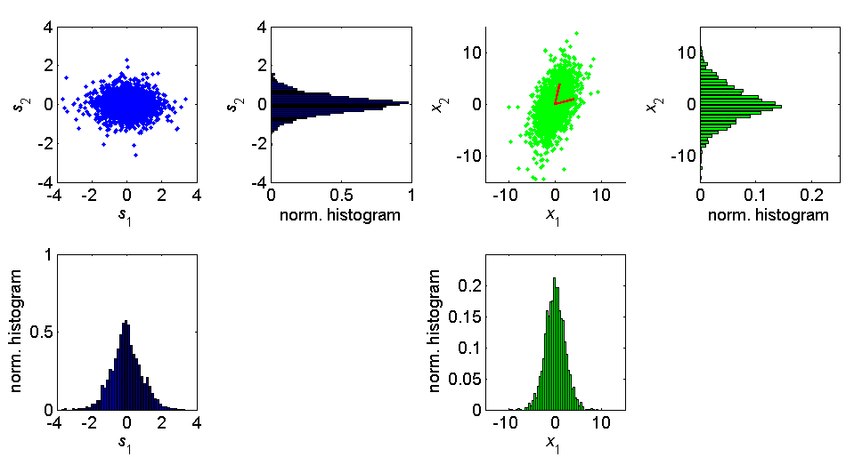
Matlab code used to generate this figure is here: LT_FIG.m

PCA

PCA can be used to determine the "principle axes" of a dataset, but it does not uniquely determine the basis associated with the linear model of the data,

PCA is only concerned with the second order (variance) characteristics of the data, specifically the mean, , andcovariance,

For independent sources combined linearly, the covariance matrix is just (assuming zero mean),

where is the diagonal matrix of source variances.Thus any basis, , satisfying,

will lead to a covariance matrix of . And sincethe decorrelating matrices are all determined solely based on the covariance matrix, it is impossible to determine a unique linear basis from the covariance alone. Matrices, unlike scalar real numbers, gnerally have an infinite number of "square roots". See Linear Representations and Basis Vectors for more information. As shown in that section, PCA can be used to determine the subspace in which the data resides if it is not full rank.

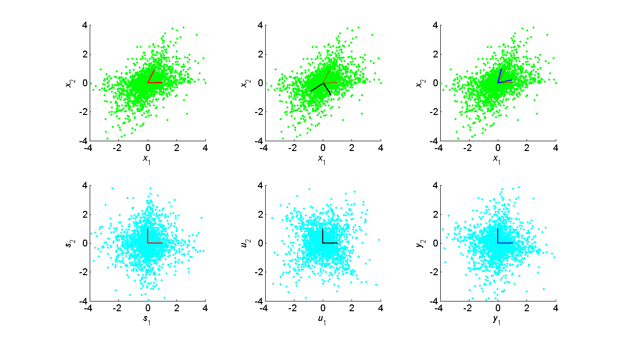
To further illustrate the non-uniqueness of the PCA basis, consider the following figure in which (i.e. Laplacian)sources are combined with the linear matrix,

N = 2000;
A = [1 2 ; 4 0.1];
A(:,1)=A(:,1)/norm(A(:,1));
A(:,2)=A(:,2)/norm(A(:,2));
s = gg6(2,N,[0 0],[1 3],[1 1]);
x = A*s;

We produce two sets of decorrelated sources, one that simply projects onto the eigenvectors, and the other which uses the unique symmetric square root "sphering" matrix (see Linear Representations and Basis Vectors for more detail.)

[V,D] = eig(x*x'/N);
Di = diag(sqrt(1./diag(D)));
u = Di * V' * x;
y = V * Di * V' * x;

Similarly for sources,

s = gg6(2,2000,[0 0],[1 3],[10 10]);
x = A*s;

Gaussian sources, unlike non-Gaussian sources, are completely determined by second order statistics, i.e. mean and covariance. If Gaussian random variables are uncorrelated, then they are independent as well. Futhermore, linear combinations or Gaussians are Gaussian. So linearly mixed Gaussian data is Gaussian with covariance matrix,

s = gg6(2,2000,[0 0],[1 3],[2 2]);
x = A*s;

And any of the infinite number of root matrices satisfying this equation will yield Gaussian data with identical statistics to the observed data.

As seen in the bottom row, the joint source density is radially symmetric, i.e. it "looks" exactly the same in all directions. There is no additional structure in the data beyond the source variances and the covariance. To fix a particular solution, constraints must be placed on the variance of the sources, or the norm of the basis vectors. However, this generally cannot be done since the ICA model assumes only independence of the sources. The source or basis vector norm is usually fixed, which determines the magnitude of the non-fixed variance or norm.

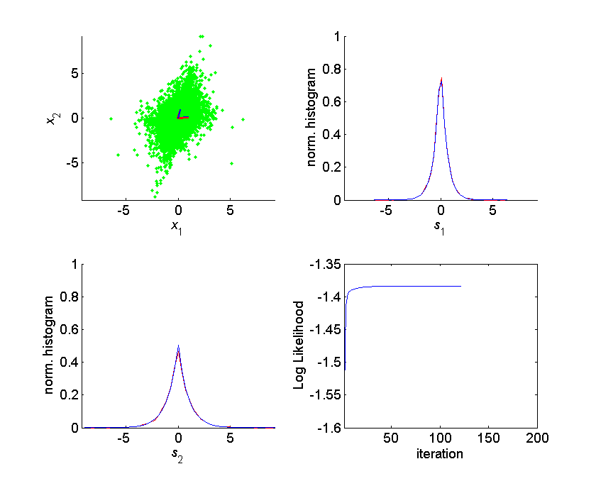
Fortunately, real sources are usually non-Gaussian, so if the ICA model holds and the sources are independent, then there is a unique basis representation of the data such that the sources are independent.

Basic ICA

Let's take some two dimensional data following the ICA model.

s = gg6(2,2000,[0 0],[1 3],[1 1]);
A = [1 2 ; 4 0.1];
x = A*s;

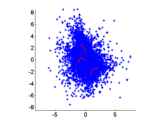
The program amica_ex.m will be used to illustrate ICA using the Amica algorithm. The output is shown below:

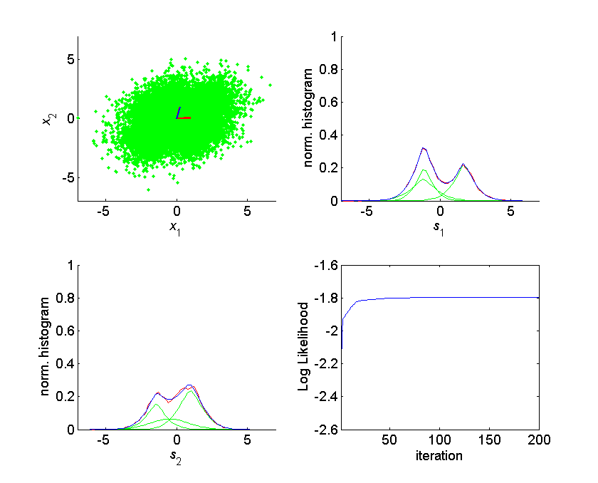
We can also experiment with multimodal sources using the function ggrandmix0.m:

s = ggrandmix0(2,20000,3); % random 2 x 20000 source matrix, with 3 mixtures in each source density
x = A*s;

Multiple Models

In the same way we created complex mixture source densities by combining a number of Generalized Gaussian constituent densities, we can create a complex data model by combining multiple ICA models in an ICA mixture model. The likelihood of the data from a single time point, then is given by,

where are the mixing matrixand density parameters associated with model .

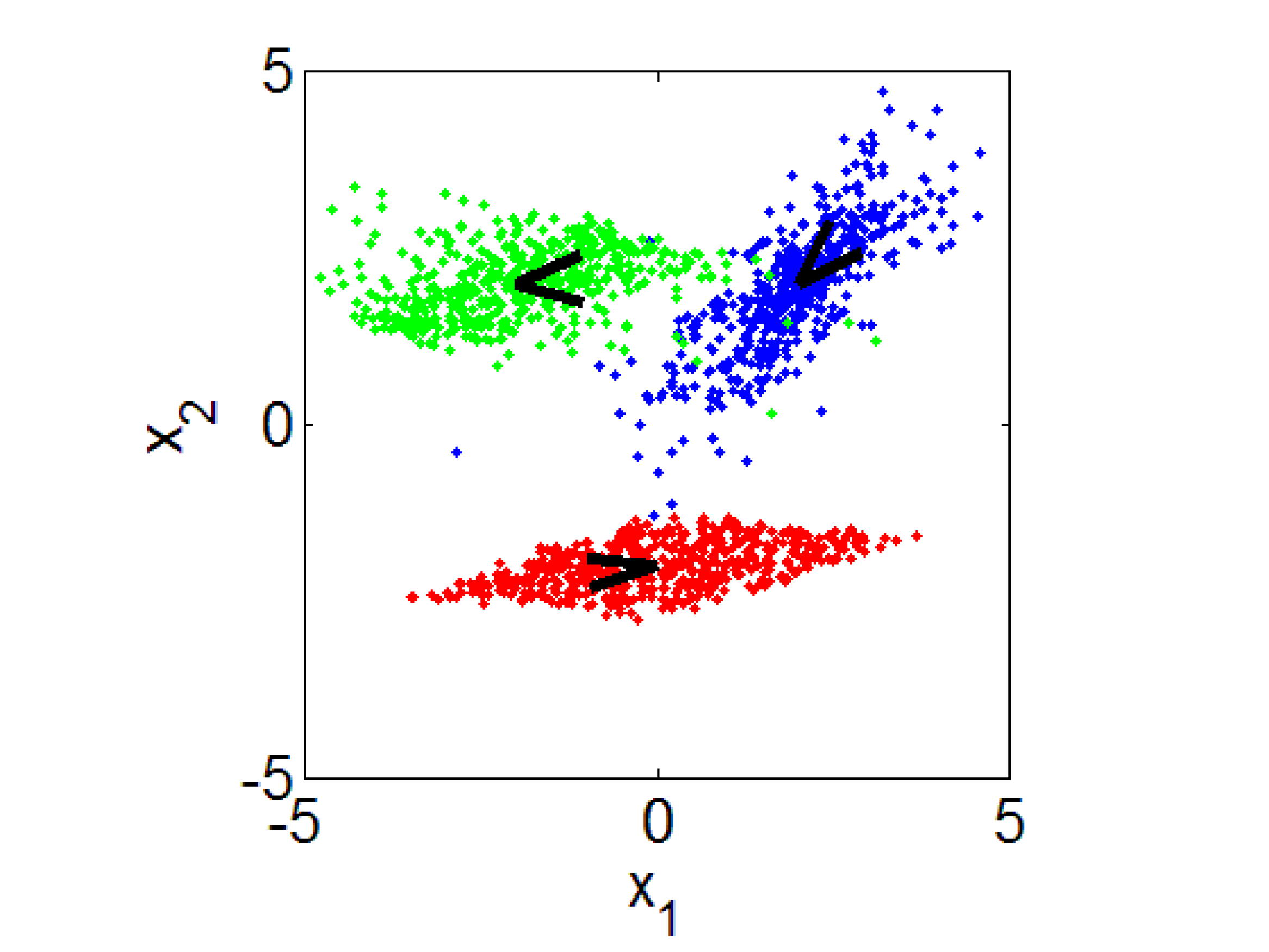
We can use the program ggmixdat.m to generate random ICA mixture model data with random Generalized Gaussian sources:

[x,As,cs] = ggmixdata(2,2000,3,[1 1; 1 1],ones(2,2),2);

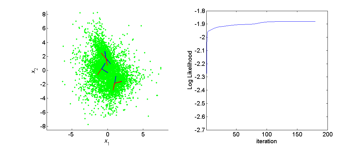
We use the program amica_ex.m to illustate:

[A,c,LL,Lt,gm,alpha,mu,beta,rho] = amica_ex(x,3,1,200,1,1e-6,1,0,1,As,cs);

The output is shown below:

Given a mixture model, we can use Bayes' Rule to determine the posterior probability that model generated the data at time point be the index of the model active at time point given, we have,

A plot of the posterior log likelihood given each model is shown below.