Matplotlib add-on to make stereograms and anaglyphs.

Stereographic images can significantly enhance the interpretability of 3D data by leveraging human binocular vision. Instead of looking at a flat projection on a page, stereograms give us "3D glasses" for 2D data with just our eyes.

It takes some practice to be able to view the stereoscopic effect for the first time, but the effort is well worth it!

Basic Usage

Python Installation

pip install mpl_stereo

Setup

from mpl_stereo import AxesStereo2D, AxesStereo3D, AxesAnaglyph
from mpl_stereo.example_data import trefoil
x, y, z = trefoil()  # trefoil knot

2D Stereogram plots

Currently, only a subset of matplotlib's 2D plots are officially supported. See the list in axstereo.known_methods.

axstereo = AxesStereo2D()
axstereo.plot(x, y, z, c='k', alpha=0.2)
axstereo.scatter(x, y, z, c=z, cmap='viridis', s=10)

When you are viewing the stereogram properly, you should see the knot weave in and out of the page!

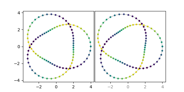
Warning: Please note that for 2D plots the stereoscopic effect requires shifting data, so the data will not necessarily line up with the x-axis labels! Right now this is controlled with the eye_balance parameter. Calling AxesStereo2D(eye_balance=-1) (the default) will ensure that the left x-axis data is not shifted, whereas AxesStereo2D(eye_balance=1) will lock down the right x-axis data. The tick labels for x-axes where the data is not aligned will have transparency applied. So in the plot above, the right side labels being lighter gray indicates that you should not trust that x-axis data to be positioned correctly, but the left subplot with its black labeling is accurate.

3D Stereogram plots

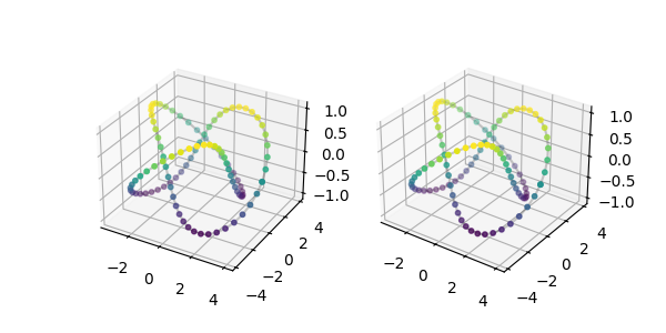
The stereoscopic effect in 3D is made just by rotating the plot view, so all of matplotlib's 3D plot types are supported, and there are no concerns about data not lining up with the axis labels.

axstereo = AxesStereo3D()
axstereo.plot(x, y, z, c='k', alpha=0.2)
axstereo.scatter(x, y, z, c=z, cmap='viridis', s=10)

Red-Cyan Anaglyphs

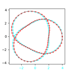
Some 2D plots can also be made into anaglyphs, which are stereograms that can be viewed with red-cyan 3D glasses. While this allows for seeing the stereoscopic effect without training your eyes, it also means that the data cannot be otherwise colored.

The same warning as for the 2D stereo plots about shifting data applies here as well. If eye_balance is -1 or +1 such that the data for one of the colors is not shifted, then that color will be applied to the x-axis tick labels to show that they are accurate.

axstereo = AxesAnaglyph()
axstereo.plot(x, y, z)
axstereo.scatter(x, y, z, s=10)

Existing Stereo Images

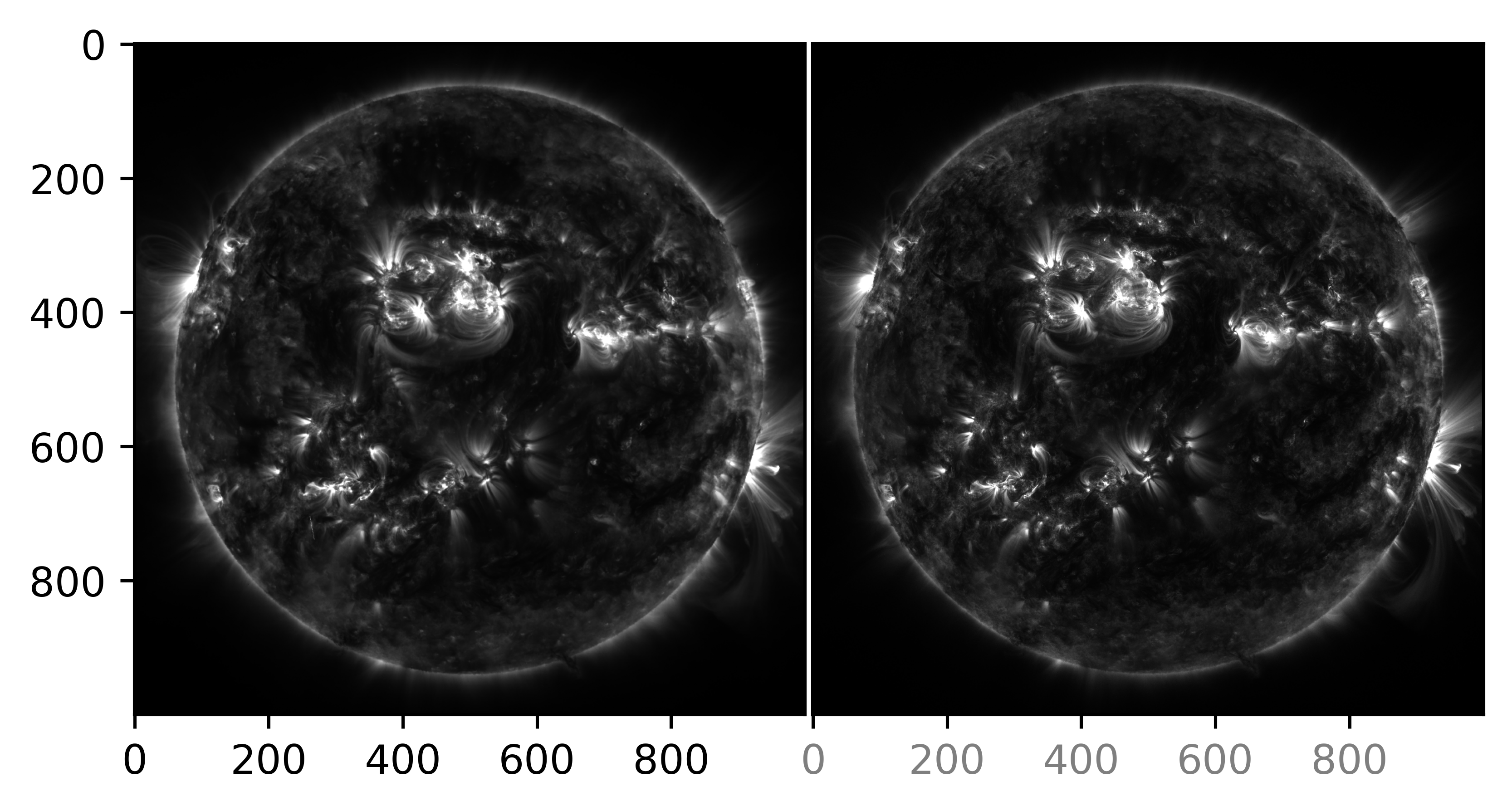
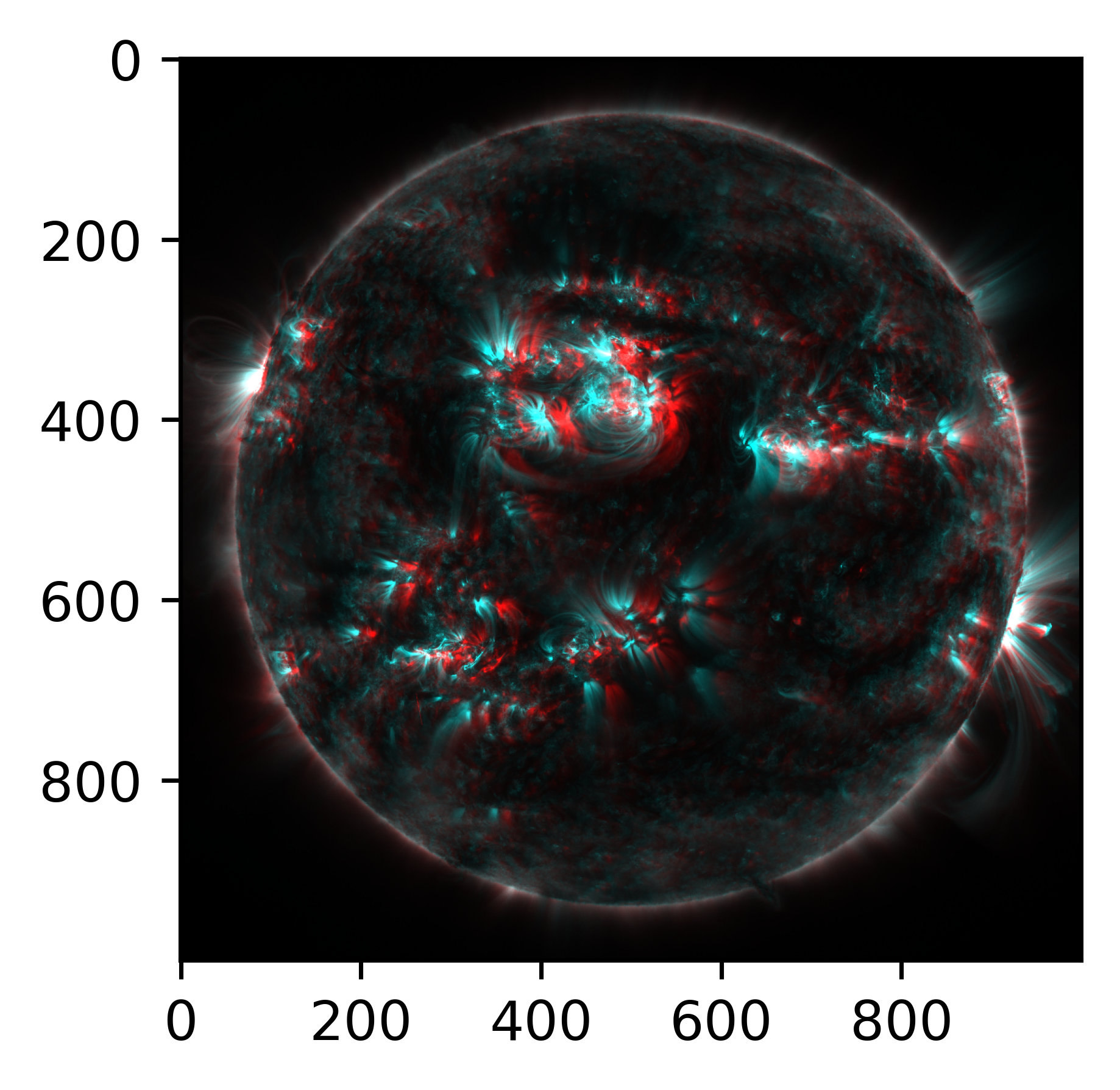
Existing stereo image data can easily be plotted up side-by-side, or combined into an anaglyph. Here we plot up two 1-D grayscale images of the sun taken in July 2023 by the NASA STEREO-A and SDO spacecraft. This example was adapted from the SunPy documentation.

from mpl_stereo.example_data import sun_left_right
sun_left_data, sun_right_data = sun_left_right

axstereo = AxesStereo2D()
axstereo.ax_left.imshow(sun_left_data, cmap='gray')  # try other colormaps!
axstereo.ax_right.imshow(sun_right_data, cmap='gray')

axstereo = AxesAnaglyph()
axstereo.imshow_stereo(sun_left_data, sun_right_data, cmap='gray')

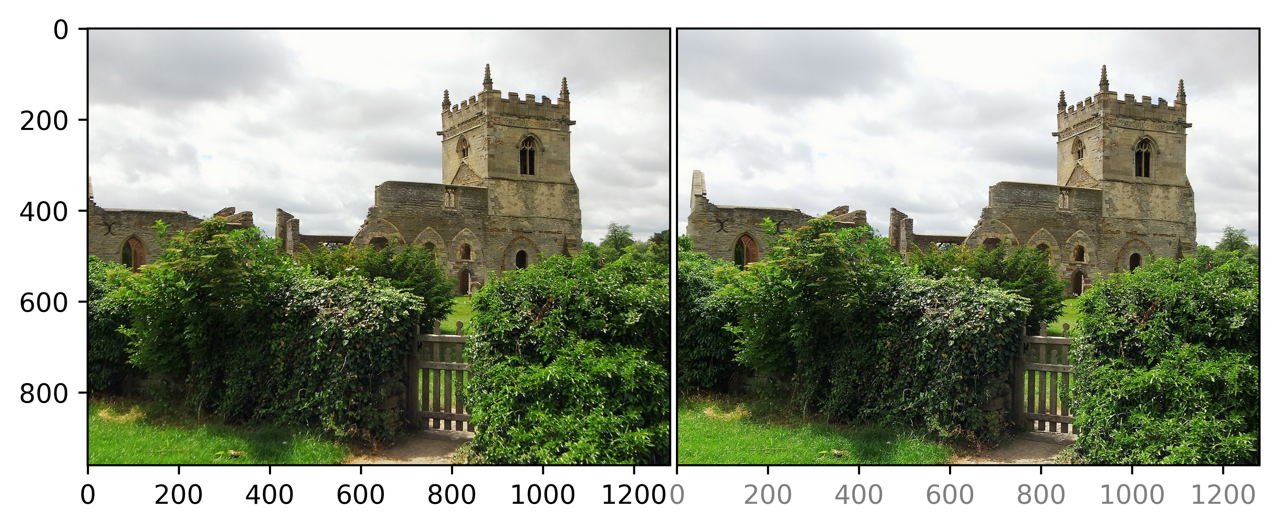
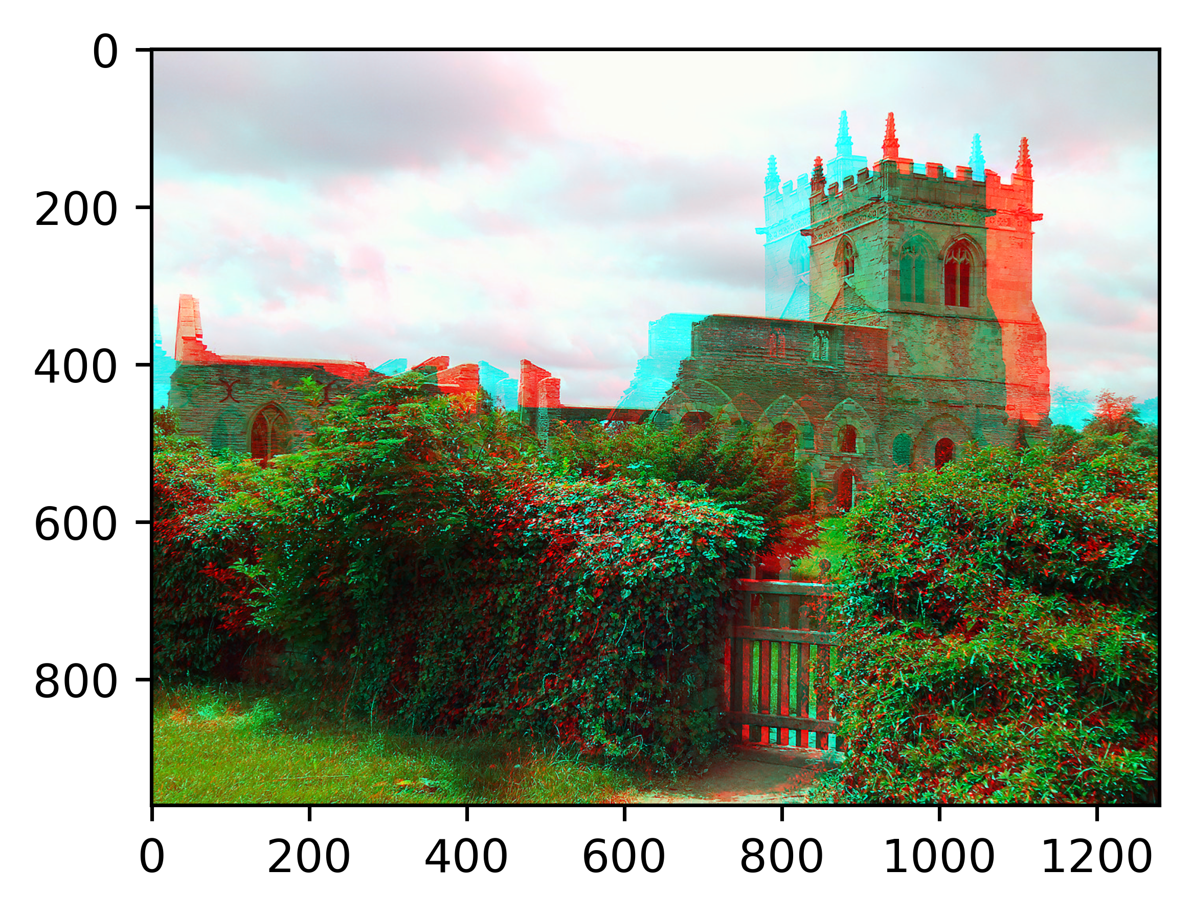
Here's another example, showing how this translates to full color data. This example is a pair of photos of St. Mary's Church in Colston Basset, Britain, taken by David Skinner and shared under a CC-BY2.0 license.

Color anaglyph algorithms can be chosen from the methods 'dubois', 'photoshop', and 'photoshop2', as described in the paper Sanders, William R., and David F. McAllister. "Producing anaglyphs from synthetic images." Stereoscopic displays and virtual reality systems X. Vol. 5006. SPIE, 2003.

from mpl_stereo.example_data import church_left_right
church_left_data, church_right_data = church_left_right

# or
import matplotlib as mpl
church_left_data = mpl.image.imread('church_left.jpg')
church_right_data = mpl.image.imread('church_right.jpg')

axstereo = AxesStereo2D()
axstereo.ax_left.imshow(church_left_data)
axstereo.ax_right.imshow(church_right_data)

axstereo = AxesAnaglyph()
axstereo.imshow_stereo(church_left_data, church_right_data)

Wiggle Stereograms

As a final way to show off the stereoscopic effect, we can make a wiggle stereogram or "wigglegram". This isn't as useful for examining data, but allows seeing the effect without having to train your eyes or using 3D glasses. The sense of depth may be enhanced if you close one eye.

axstereo = AxesStereo2D()  # wiggle also works with AxesStereo3D
axstereo.ax_left.imshow(sun_left_data, cmap='gray')
axstereo.ax_right.imshow(sun_right_data, cmap='gray')
axstereo.wiggle('sun_wiggle.gif')  # saves to file

Advanced Usage

Working With Plots

The figure and subplot axes can be accessed with the following:

axstereo.fig
axstereo.axs  # (ax_left, ax_right), for AxesStereo2D and AxesStereo3D
axstereo.ax  # for AxesAnaglyph

Calling any method on axstereo will pass that method call onto all the subplot axes. In the 2D cases, the plotting methods which take in x and y arguments are intercepted and the additional z data is processed to obtain appropriate horizontal offsets.

# For example instead of:
for ax in axstereo.axs:
    ax.set_xlabel('X Label')

# You can do the equivalent:
axstereo.set_xlabel('X Label')

# When applicable, the return values from the two method calls are returned as a tuple
(line_left, line_right) = axstereo.plot(x, y, z)

Parallel vs Cross-Eyed Viewing

By default, the stereograms are set up for the "parallel" / "divergent" / "wall-eyed" viewing method. For "cross-eyed" viewing, initialize with a negative ipd parameter. An ipd (Inter-Pupilary Distance) of 65 millimeters is the default, so call AxesStereo2D(ipd=-65) for the default cross-eyed viewing.

Depth and Focal Plane Location

The apparent depth of 2D stereograms can be adjusted with the zscale parameter. The default is 1/4th the x-axis range, i.e. zscale=(max(ax.get_xlim()) - ax.get_xlim()) / 4. Decrease this number to flatten the stereogram, or increase it to exaggerate the depth.

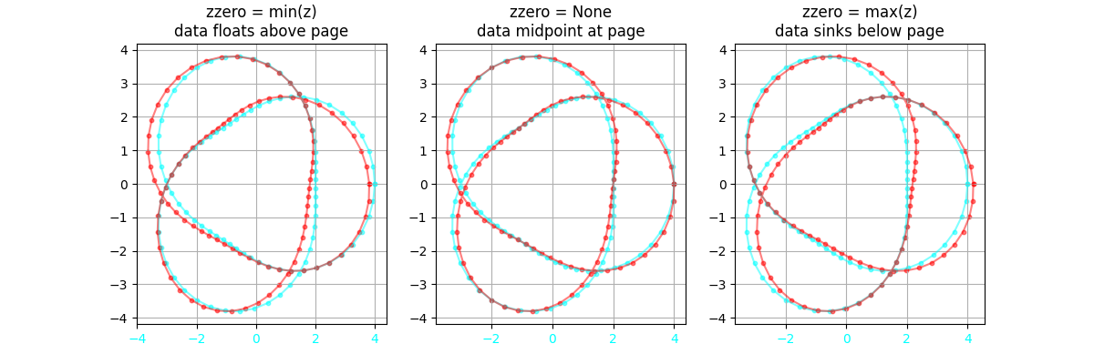
For 2D plots and anaglyphs, the focal plane can be set with the zzero parameter. This is the z value that will be "on the page" when viewing the stereogram.

axstereo = AxesAnaglyph(zzero=min(z))  # data will float above the page
axstereo = AxesAnaglyph(zzero=None)  # page will be at the midpoint of the data range (default)
axstereo = AxesAnaglyph(zzero=max(z))  # data will sink below the page

Animations

See an example of how to use this with matplotlib animations in docs/gen_graphics.py.

Viewing Stereograms

These are not autostereograms, like the "Magic Eye" books that were popular in the 1990's. However, they use the same viewing technique. Below is a great video by Vox on how to view stereograms, click on the image and skip to 0:35 for the how-to portion and then 4:33 for more examples.

There is also a great how-to guide at the stereoscopy blog here: Learning to Free-View: See Stereoscopic Images with the Naked Eye

Derivation of Geometry

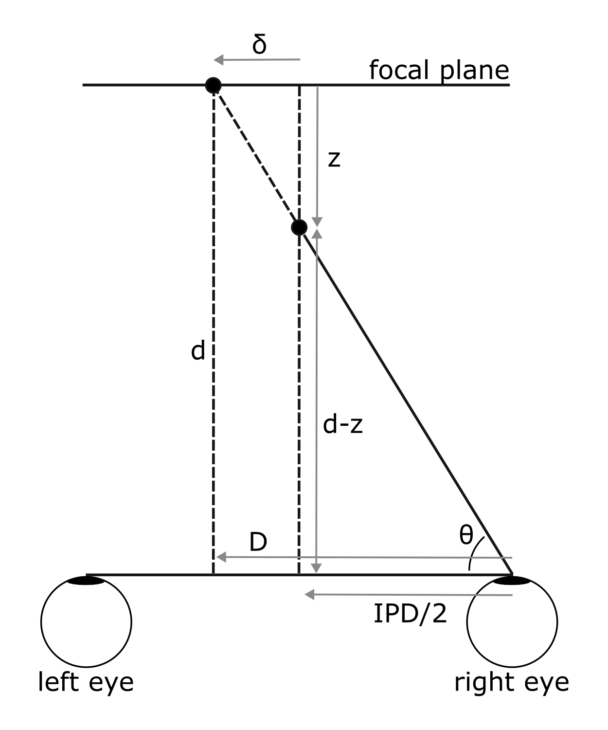
Two eyes with separation IPD are looking at a point a distance z offset from a focal plane at distance d, resulting in view angle θ. If this point were projected back to the focal plane, it would be offset by δ from where it visually appears on that plane. This offset δ is used to displace each point in the 2D stereograms and anaglyphs for each eye based on its z value to achieve the stereoscopic effect. The eye_balance parameter allocates the total relative displacement of 2δ between the two eyes.

For 3D stereograms, the azimuth view angle for the two plots is simply shifted by θ, with no modification to the data.

θ = arctan((d - z) / (IPD / 2))
D / d = (IPD / 2) / (d - z)
δ = D - IPD / 2
  = IPD / 2 * (d / (d - z) - 1)
  = IPD / 2 * z / (d - z)