Table of Contents

1. About The Project
   • Background
   • Motivation
2. Getting Started
   • Prerequisites
   • Folder Structure
   • Installation
3. Usage
• Tests
4. Acknowledgments
5. Requirements

About The Project

Background

This project is inspired by Boutet, A., Madhavan, R., Elias, G.J.B. et al. (2021), an investigation on finding optimal parameters for deep brain stimulation. This model is applicable to parameter recovery within the Hodgkin Huxley model.¹ It is applicable to multiple forms of real world data, but has a preloaded L5PC neuron and redumentary Hodgkin Huxley Neuron. Given the project scope, the user can specify two main objectives: to recover the impulse used to stimulate the neuron or to recover the specific instance parameters of the Hodgkin Huxley.

Slide Deck

The L5PC Neuron

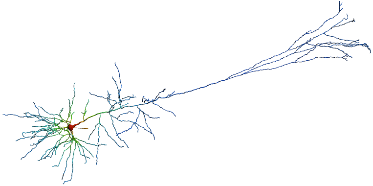
A model of the L5PC neuron was adopted from Hay, Etay, et al. (2011).² See Repo Layer 5 (L5) neurons are the fundamental output layer of cortical structures and consist of 2/3 of the mammilian cortex. When characterizing behavior, neuroscientists largely attribute cognitive processings to occur in L5PC neurons. Our L5 consists of long-range projection pyramidal neurons signaling a columnar output to both cortical and extracortical regions of the brain. Recent literature, Moberg S, Takahashi N. (2022), has suggested two subclasses of morphologically distinct L5 neurons exist. These differences cause subsequent distinct electrophysiological properties.³ However, traditionally, computational models of neurons neglect these distinguishers. This leads to the question, can one use simplified computational models such as the Hodgkin Huxley to recovor more complex behaviors of the L5PC neuron? If so, is this accurate; and is it possible to optimize the computational model of such a neuron to closely fit the desired result, while maintaining biological feasibility?

Hodgkin Huxley Model

For implementation, a Biophysical model (i.e., a Hodgkin-Huxley model) is used, based on: Izhikevich, Eugene M. Dynamical systems in neuroscience

The Adjoint Method

Define a nonlinear system $V(t+1) = \mathbf{F}(V(t))$ where $t \in [0, T]$ and operator $\mathbf{F}$ solves the Hodgkin-Huxley system of ODEs using the forward Euler method. We are interested in finding an optimal value of some uknown parameter $m$ that minimizes a cost function $J$. This optimization problem can be solved using the Lagrange multiplier technique. Let $\mu(t)$ be a Lagrange multiplier and define the Lagrangian as $$\mathcal{L} = J - \sum_{k=1}^{T} \mu(k)[V(k) - \mathbf{F}(V(k-1))]$$ Note that on the equations of motion (i.e. when $V(t) = \mathbf{F}(V(t-1))$ ), derivatives of $\mathcal{L}$ are equal to derivates of $J$. Thus, by construction of the Lagrangian, $\frac{\partial \mathcal{L}}{\partial m}$ on the equations of motion occurs at the minima. In order to find the minima, we first compute gradients using autograd, an Automatic Differentiation python library, and then search for a minimum using scipy's optimization library.

Implementing a Neural Network

In general, neural networks are comprised of node layers containing an input layer, one or more hidden layers, and an output layer. Each node connects to those in the previous layer with an associated weight; calculations are performed between nodes that mimic that passing of signals from one biological neuron to another. Together, these hidden layers and nodes can be trained and their parameter’s adjusted to learn data: identify patterns, predict data, etc.

For this application, the objective is to optimize a neural network to recover the amplitude and waveform of an impulse from neuronal voltage time series data given a known underlying dynamical system.

Motivation

While this project presents a fundamental assessment of this problem, further expansions could play critical roles in disease treatments, such as in dementia and epilepsy.⁴⁵

Getting Started

Prerequisites

For proof of concept, we recommend looking at the JupyterNotebooks in .\development\tests. For sample implementation of an adjoint class refer to .\adjoint\stim_adj_test.ipynb. For sample neural network implimentation refer to .\neuralnet\NN-training-example.ipynb .

Note: The class implementations have a more significant runtime due to variable storage and high runtime overhead. Additionally, a class implementation has high method lookup overhead and overhead due to accessing global variables. Future directions would implement further runtime analysis, and likely the reworking of classes into python scripts.

Folder Structure

.
├── adjoint                      # All Api for adjoint based parameter recovery
├── development                  # build folder
  ├── models                     # All ipynb towards implimenting inverse problems
  ├── tests                      # Test files -- samples
  ├── runtime            
├── images                       # res (static images)
├── neuralnet                    # All Api for neural network parameter recovery and waveform fitting
├── sim_data                     #src files
  ├── HH_data                    
  ├── models                     # neuronal type files
  ├── mods                       # mod folders containing conductance mechanisms
  ├── morphologies               # neuronal morphology designation
  ├── tests
  ├── x86_64                     #executables (C) 
├── .DS_Store
├── .gitignore
├── NEURON_inst.py               # NEURON dependencies
├── README.md
├── requirements.txt             # file dependencies
└── upload.py                    #API for file retrieval

Installation

Minimal working example and getting started:

1. Clone the repo:

   git clone [git@github.com:sepstein22/computational_brain.git]

2. Go into the Directory:

   cd computational_brain

3. Install Dependencies:

   pip install -r requirements.txt

To run adjoint methods:

4. Go into Adjoint Directory;

cd adjoint

4. Create an instance of the file fetching class:

   python3
   import sys
   import os
   sys.path.append('../')
   from stim_adj import stim_adj
   from upload import retrieve_file
   #neuron_type = , num_ap = 
   inst_file = retrieve_file(neuron_type, num_ap)

5. Load the Data:

   V_data, I_data, t_data, V0, dt, b = inst_file.load()

6. Create an instance of the solver class:

   #HH_params = , guess_a = , guess_c =
   I_params, V = instance.recovery()

7. Visualize the results.

For more complex implementations (we do not recommend currently doing this, as it has poor runtime performance and some intermittent convergence issues):

Follow steps 1-3:

4. Create an instance of the parent class:

   from param_test import ParameterRecovery
   
   inst = ParameterRecovery(known_parameters, unknown_parameters, dt, neuron_type, ...)

5. Assign parameters:

   param_list = inst.assign_parameters()
   bounds = inst.define_bounds()
   init_guess = inst.def_guess_params()

6. Call optimizer:

   optim_sol = inst.optimize()

To run neural net methods:

Please refer to section in usage.

Usage

There are several key files to run the adjoint method in this repo. Please refer to .\adjoint\stim_adj_test.ipynb and .\neuralnet\NN-training-example.ipynb for a minimal use case.

• upload.py: loads data
• .\adjoint\stim_adj.py : class to implement the forward model, cost method, adjoint method, and optimization when we are seeking to recover parameters of the Impulse wave {a: amplitude, c: frequency, b: center } assuming a guassian waveform
• .\adjoint\param_adj.py : class to implement the forward model, cost method, adjoint method, and optimization when we are seeking to recover the parameters of the Hodgkin Huxley equation with a known impulse wave {g_Na: , g_K, g_L, E_Na, E_K , E_L, C_m, m, n, h}. It assumes all these values are unknown. If any of these values are loaded in as known in the param_test file (which will be explained below), it sets both the upper and lower bounds when implementing optimization equal to this value, as well as the initial guess.
• .\adjoint\param_test : is the class the user interacts with. It calls the three files above. It takes in the following arguments:
  • known_params: a dictionary of any known values in the problem.
  • unknown_params: a dictionary of all unknown values in the problem.
  • dt : time step for simulation
  • neuron_type: This is used to retrieve file type due to our naming convention in upload.py. Type of data assumed to be one from list ['manual', 'L5PC', 'HH'].
  • num_ap: This is used to retrieve file type due to our naming convention in upload.py.
  • V_data: Is not required, but takes in a np array if the user wants to specify manual data importation.
  • I_data: Is not required, but takes in a np array if the user wants to specify manual data importation.
  • t_data: Is not required, but takes in a np array if the user wants to specify manual data importation.
  • method: Specifies the optimization method that will be loaded into stim_adj.py or param_adj.py.
  • bounds: Specifies a list of bounds. This will be updated for known values as well in the parameter optimization case.
  • tol: Specifies the optimization tol to reduce runtime.

It is assumed the parameters are given to be of the following form ['g_Na', 'g_K', 'g_L', 'E_Na', 'E_K', 'E_L', 'C_m', 'm', 'h', 'n', 'stim']. If the user includes 'stim' as an unknown all other values are assumed to be known, since we do not allow for the combination of impulse and parameter recovery.

After defining parameters, this file is broken down into a few major functoins:

1. assign_parameters acts as a test funciton to warn the user what parameters remained undefined and will be assumed to be of the standard Hodgkin Huxley Model.
2. define_bounds: defines upper and lower bounds for both problem types.
3. def_guess_params: defines initial guesses based on known and unknown values.
4. adj_impulse: calls an instance of stim_adj.py and returns the final Voltage and the optimal value of the impulse parameters [a, c].
5. adj_params: calls an instance of param_adj.py and returns the integrated for final Voltage and the optimal value of the HH parameters.
6. optimize: determines what type of problem we have and calls the sorrect adj_ function
7. graph: plots the optimal solution.

The folder specified development includes debugging processes, alternatively tested loss functions, as well as other test notebooks.

• .\neuralnet\NNengine.py: classes that store hidden layer parameters and functions necessary to create/train a neural network.
  • Run_NN: creates and runs a neural network, automatically forward and back propagating to adjust the network’s hyperparameters
• .\neuralnet\WaveformGenerator.py : contains methods to create waveform data; methods used to fit neural network output (impulse input prediction) data to a waveform.
• .\NN-training-example.py: guides users through simplest example of training a neural network, fitting its output to a waveform, and obtaining accuracy (mean squared error).

.\NN-training-example.py in summary works through:

1. Import simulation data from the ‘sim_data’ folder
2. Rescale and normalize data for neural network stability
3. Initiate a Multilayer object (the highest level object that will be encoded with all the neural network’s parameters)

NN = Multilayers(nin,nouts)
#nin (int): num of input data pts
#nouts of form [num_nodes1, num_nodes2,... num_nodesN, num_ouputs]; nout=[300, nin] (1 layer of 300 nodes and the same number of outputs as inputs)

4. Calling Run_NN on multilayers object and simulation data to output prediction/estimation of input impulse data
5. Fit output data to different waveforms from WaveformGenerator.py to return best fit and accuracy metric.

Making future predictions using a trained Neural Network requires calilng respective Multilayers objects on new impulse data:

nn_object = Multilayer(nin, outs)
nn_object(new_input, true_output_data)

Optimal neural netowrk implimentation requires training on diverse datasets and parameter/hyperparameter tuning ( nout: number of layers and nodes, step_size: defining step size for gradient descent, iter_lim: number forward and backpasses, error_thresh: limiting backpasses (preventing overfitting)).

Tests

Prior to running the model we recommend the user runs some unit tests these include:

1. Insuring there are equal time steps and data. assertEqual(len(self.V_data), len(self.t_data))
2. Finite Gradient check: instance.fd_check(1, 0) A sample plot looks like the following:

Acknowledgments

This uses the following open source packages:

• NEURON
• Autograd

Requirements

Programming dependies specified in requirements.txt

   pip install -r requirements.txt

Footnotes

1. Boutet A, Madhavan R, Elias GJB, Joel SE, Gramer R, Ranjan M, Paramanandam V, Xu D, Germann J, Loh A, Kalia SK, Hodaie M, Li B, Prasad S, Coblentz A, Munhoz RP, Ashe J, Kucharczyk W, Fasano A, Lozano AM. Predicting optimal deep brain stimulation parameters for Parkinson's disease using functional MRI and machine learning. Nat Commun. 2021 May 24;12(1):3043. doi: 10.1038/s41467-021-23311-9. PMID: 34031407; PMCID: PMC8144408. ↩

2. Hay, Etay, et al. "Models of neocortical layer 5b pyramidal cells capturing a wide range of dendritic and perisomatic active properties." PLoS computational biology 7.7 (2011): e1002107. ↩

3. Moberg S, Takahashi N. Neocortical layer 5 subclasses: From cellular properties to roles in behavior. Front Synaptic Neurosci. 2022 Oct 28;14:1006773. doi: 10.3389/fnsyn.2022.1006773. PMID: 36387773; PMCID: PMC9650089. ↩

4. Luo, Y., Sun, Y., Tian, X., Zheng, X., Wang, X., Li, W., Wu, X., Shu, B. and Hou, W., 2021. Deep brain stimulation for Alzheimer's disease: stimulation parameters and potential mechanisms of action. Frontiers in aging neuroscience, 13, p.619543. ↩

5. Lv, Q., Du, A., Wei, W., Li, Y., Liu, G. and Wang, X.P., 2018. Deep brain stimulation: a potential treatment for dementia in Alzheimer's disease (AD) and Parkinson's disease dementia (PDD). Frontiers in neuroscience, 12, p.360. ↩