Vehicle Detection Project

The goals / steps of this project are the following:

• Perform a Histogram of Oriented Gradients (HOG) feature extraction on a labeled training set of images and train a classifier Linear SVM classifier
• Optionally, you can also apply a color transform and append binned color features, as well as histograms of color, to your HOG feature vector.
• Note: for those first two steps don't forget to normalize your features and randomize a selection for training and testing.
• Implement a sliding-window technique and use your trained classifier to search for vehicles in images.
• Run your pipeline on a video stream (start with the test_video.mp4 and later implement on full project_video.mp4) and create a heat map of recurring detections frame by frame to reject outliers and follow detected vehicles.
• Estimate a bounding box for vehicles detected.

Rubric Points

###Here I will consider the rubric points individually and describe how I addressed each point in my implementation.

###Spatial and Histogram Features

The spatial features are extracted with bin_spatial function in the code cell 10. The histogram features are extracted with color_hist function in the code cell 11. In order to find the best spatial and histogram parameters, 5-fold cross validation was performed over the subset images. The subset images have 1196 car images and 1125 notcar images. The code is in the spahist.py file. Several sets of parameters was tested. The tested parameters, selected parameters according to highest average accuracy, and the parameter set that has the highest average accuracy over 5-fold are given in the following table.

Spatial (Test)	Histogram (Test)	Spatial	Histogram	Best	Acc
8,16,32,64,128	8,16,32,64,128	8,16,32	128,64,32	16,32	0.9897
8,12,16,24,32	32,48,64,96,128	12,16,32	128,96,64	12,32	0.9905
8,10,12,14,16	64,96,128,192,256	12,14,16	64,96,128	12,96	0.9935
12,13,14,15,16	64,80,96,112,128	12,13,16	96,112,128	12,112	0.9935
11,12,13,14,15,16	100,114,128,142,156	14,15,16	114,128,142	14,142	0.9919
11,12,13,14,15,16	100,114,128,142,156	12,14,16	100,114,142	14,100	0.9940

The highest accuracy depends on the data; however, a spatial value between 12 - 16 performed better. The number of bins value did not have that much effect on the accuracy value. Values greater than 32 performed usually better than the values smaller than 32. Usually, 128 used to perform following tests.

###Histogram of Oriented Gradients (HOG)

####1. Extracting HOG features from the training images.

Hog features are extracted as in the 9th code cell of the Ipython notebook. First, the image is converted to desired color space, then each channel of the image is sent to hog function of skimage.feature module. The required parameters are orient, pix_per_cell and cell_per_block. The helper function is the get_hog_features function in code cell 7.

Here is an example using one of the best parameter set for extracting hog features, the YCrCb color space and HOG parameters of orientations=9, pixels_per_cell=(8, 8) and cells_per_block=(2, 2):

####2. Explain how you settled on your final choice of HOG parameters.

#####2.1. Comparison 1 Similar 5-fold test was performed for hog parameters on the subset images data set. The parameters used in this experiment are as follows:

• Colorspace : HLS, HSV, LUV, RGB, YCrCb, YUV
• Orient: 6, 9, 12
• Pix Per Cell (PPC): 4, 6, 8, 10, 12
• Cell Per Block (CPB): 1, 2 ,3 ,4
• Hog Channel (HOGCH): 0, 1, 2, ALL

The top ten performing parameter sets are given in the following table.

Color	Orient	PPC	CPB	HOGCH	HOGsec	TRNsec	Acc
HLS	12	4	2	ALL	26.958	1.494	0.9970
HSV	12	4	1	ALL	28.722	0.412	0.9966
YCrCb	6	4	3	ALL	23.835	1.492	0.9961
YCrCb	6	4	4	ALL	21.723	2.24	0.9961
HLS	12	4	3	ALL	25.159	2.916	0.9961
HLS	12	4	1	ALL	28.297	0.396	0.9961
HLS	12	6	1	ALL	14.959	0.168	0.9957
YUV	6	4	4	ALL	21.394	2.236	0.9957
HSV	12	4	2	ALL	27.452	1.484	0.9957
HSV	12	6	1	ALL	15.236	0.162	0.9952

The best performing parameter that can be determined was only the ALL of the hog channels.

Since this test and the previous test on spatial parameters and histogram parameters are not sufficient to select hog parameters, other tests combining all parameters are performed.

#####2.2. Comparison 2 The changes can be listed as follows:

• Dataset changed to the complete data set which contains 8792 cars and 8968 notcars.
• 5-fold cross validation changed to 5x2-fold cross validation. Therefore, for each fold half of the data is used for training and the other half is used for testing.
• imreader was added as a new parameter, which indicates the module to be used to read images. Since mpimg reads images as they have a pixel value between 0 and 1, it affected the classifier performance.

For the following comparison, only cv2 was used as image reader. The parameters used in this experiment are as follows:

• Colorspace : HSV, LUV, YCrCb, YUV
• Orient: 8, 9, 10, 11, 12
• Pix Per Cell (PPC): 4, 6, 8, 10, 12, 14, 16
• Cell Per Block (CPB): 1, 2
• Hog Channel (HOGCH): ALL The top 15 parameter sets are given in the following table. The HOGsec column shows the feature extraction time.

Color	Orient	PPC	CPB	HOGsec	TRNsec	TESTsec	Acc
YCrCb	12	8	2	86.96	2.436	0.0006	0.9891
YUV	12	8	2	86.7	2.503	0.0017	0.989
YCrCb	12	4	2	215.8	6.5	0.0022	0.9883
YCrCb	10	8	2	85.68	2.906	0.0015	0.9882
YUV	12	4	2	212.62	6.465	0.0013	0.988
YUV	10	8	2	84.66	1.416	0.0003	0.9878
YCrCb	10	4	2	212.89	5.579	0.0016	0.9876
YCrCb	11	4	2	215.36	6.152	0.0025	0.9876
YCrCb	11	8	2	86.37	5.403	0.0023	0.9875
YUV	10	4	2	205.88	5.481	0.0015	0.9874
YCrCb	12	4	1	225.85	2.002	0.0016	0.9874
YUV	12	4	1	223.39	1.972	0.0011	0.9871
YUV	11	8	2	85.3	1.525	0.0023	0.987
LUV	10	4	2	201.01	6.027	0.0006	0.987
YCrCb	9	8	2	83.47	5.304	0.0012	0.9869

#####2.3. Comparison 3 Another comparison was performed to determine whether the spatial parameter or the number of bins parameter affect the accuracy when three methods are combined. In addition, the effect of changing the image reader was tested. The parameters used in this experiment are as follows:

• imreader: cv2, mpimg
• Colorspace : YCrCb, YUV
• Orient: 6, 9, 12
• Pix Per Cell (PPC): 16
• Cell Per Block (CPB): 1, 2, 3
• Hog Channel (HOGCH): 0, 1, 2, ALL
• Spatial (Spa): 8, 12, 14, 16, 32
• Number of Bins(Hbin): 64, 114, 128, 142, 192

#	imreader	Color	Orient	CPB	HOGCH	Spa	Hbin	FeatVLen	HOGsec	TRNsec	TESTsec	Acc
1	cv2	YCrCb	12	1	ALL	16	114	1686	72.56	1.296	0.0186	0.994
2	cv2	YUV	12	1	ALL	16	114	1686	72.03	1.691	0.0181	0.994
3	cv2	YUV	12	1	ALL	16	128	1728	72.22	1.594	0.0165	0.994
4	cv2	YUV	12	1	ALL	12	114	1350	73.23	1.343	0.0121	0.9939
5	cv2	YCrCb	12	1	ALL	16	128	1728	72.82	1.336	0.0179	0.9939
6	cv2	YUV	12	1	ALL	12	128	1392	72.64	1.021	0.0119	0.9939
7	cv2	YCrCb	12	1	ALL	14	114	1506	72.57	1.22	0.0126	0.9938
8	cv2	YCrCb	12	1	ALL	12	114	1350	72.47	1.218	0.0114	0.9938
9	cv2	YUV	12	2	ALL	12	192	2304	68.75	2.144	0.021	0.9938
10	cv2	YUV	12	1	ALL	16	64	1536	72.17	1.298	0.0222	0.9938
11	cv2	YUV	12	2	ALL	14	192	2460	68.67	1.556	0.0211	0.9937
12	cv2	YCrCb	12	1	ALL	16	142	1770	73.08	1.541	0.0162	0.9937
13	cv2	YUV	12	1	ALL	16	192	1920	72.41	1.987	0.0169	0.9937
14	cv2	YUV	12	2	ALL	14	114	2226	68.07	2.166	0.0229	0.9937
210	mpimg	YCrCb	12	1	ALL	12	192	1584	64.52	1.539	0.0149	0.9921

As a result, cv2 (0.9799) performed better than mpimg (0.9759) as image reader. It had both higher average and the best performing parameter set with mpimg read come 210th. It is hard to differentiate Hbin values from each other, but the spatial values between 12 and 16 mostly performed better than 8 and 32.

#####2.4. Comparison 4 There were other tests applied. The effect of using the original image on spatial and histogram feature extraction whereas using YCrCb on hog feature extraction was tested. Both of them affected to have lower accuracy. The decrease on accuracy when changing the color space for histogram feature extraction was higher, from 0.9912 to 0.9893. For spatial feature extraction, the decrease was from 0.9905 to 0.9901.

#####2.5. Comparison 5

The performance of ensembling was tested in another comparison. Three SVMs were trained with spatial features, histogram features, and hog features. The classification was performed by majority voting. The ensemble usually performed better than all of the classifiers separately, however combining all features and training one SVM outperformed ensembling. The reason for that is, the SVM with hog features has much more accuracy that the others. When ensembling, the samples correctly classified by the hog SVM were classified wrong. The parameters used in this experiment are as follows:

• imreader: cv2
• Colorspace : YCrCb, YUV
• Orient: 9
• Pix Per Cell (PPC): 4, 8, 16
• Cell Per Block (CPB): 1, 2
• Hog Channel (HOGCH): ALL
• Spatial (Spa): 12, 14, 16
• Number of Bins(Hbin): 114, 128, 142

The average accuracy values for the ensemble, combined, and separate SVMs are given in the following table.

Features	Accuracy
All	0.9924
Ensemble	0.9858
Hog	0.9822
Hist	0.9367
Spatial	0.9137

#####2.6. Comparison 6

The results shown in the following table belong to the search for the models with high accuracy, and for the models with relatively high accuracy and low feature extraction time.

#	imreader	Orient	PPC	CPB	HOGCH	FeatVLen	HOGsec	TRNsec	TESTsec	Acc
1	cv2	12	8	1	ALL	3456	106.87	2.959	0.0322	0.9943
2	cv2	12	8	2	ALL	8208	100.72	1.507	0.0731	0.994
3	cv2	12	12	1	ALL	2052	78.04	1.971	0.0204	0.9935
4	cv2	12	16	1	ALL	1728	72.43	1.79	0.0159	0.9935
5	cv2	12	16	2	ALL	2448	69.3	2.289	0.024	0.9934
6	cv2	9	8	2	ALL	6444	94.05	4.263	0.0574	0.9934
7	cv2	9	8	1	ALL	2880	103.16	2.317	0.026	0.9933
8	cv2	9	16	2	ALL	2124	66.32	1.616	0.0324	0.9932
9	cv2	12	12	2	ALL	3456	71.25	1.865	0.0344	0.9929
10	cv2	9	16	1	ALL	1584	70.11	1.712	0.0156	0.9929
-	cv2	9	16	1	0	1296	35.34	1.323	0.0116	0.9886
-	cv2	12	16	1	0	1344	35.88	1.369	0.0117	0.9889
-	cv2	6	16	2	0	1368	33.14	1.664	0.0127	0.986
-	cv2	12	12	1	0	1452	37.77	1.727	0.0132	0.988
-	cv2	9	12	1	0	1377	37.11	1.624	0.0138	0.9874
-	cv2	9	12	2	0	1728	34.55	2.103	0.015	0.9885
-	cv2	9	16	2	0	1476	33.78	1.567	0.0151	0.9889
-	cv2	6	8	1	0	1536	45.19	1.758	0.0153	0.9876
-	cv2	9	8	1	0	1728	46.27	2.229	0.0162	0.9899
-	mpimg	12	8	1	0	1920	45.41	2.464	0.0166	0.9864
-	mpimg	9	8	1	0	1728	45.07	2.244	0.0175	0.987

The parameters used in this experiment are as follows:

• imreader: cv2, mpimg
• Colorspace : YCrCb
• Orient: 6, 9, 12
• Pix Per Cell (PPC): 8, 12, 16, 24, 32
• Cell Per Block (CPB): 1, 2
• Hog Channel (HOGCH): 0, 1, 2, ALL
• Spatial (Spa): 16
• Number of Bins(Hbin): 128

#####2.7. Comparison 7

After trying the models on the project video, and switching to multiple scale windows the time required to process the video was considerably high. In order to decrease the time to process the video, the time spend on each feature extraction process was investigated. HOG features can be extracted in the beginning for each frame and each scale value. The most time-consuming operation is to extract the histogram features for a frame. Since it is required to process each window separately. As a result, models without histogram features were examined. In addition, in previous experiments, the 0 and 1 hog channels for YCrCb and 0 and 2 hog channels for YUV performed better the remaining hog channel.

#	Color	Orient	PPC	CPB	HOGCH	FeatVLen	HOGsec	TRNsec	TESTsec	Acc
1	YUV	12	8	2	[0- 1- 2]	7824	87.1	1.562	0.0684	0.9926
2	YCrCb	12	8	2	[0- 1- 2]	7824	88.21	2.73	0.0673	0.9926
3	YCrCb	12	8	2	[0- 1]	5472	60.82	1.975	0.0495	0.9919
4	YCrCb	10	8	2	[0- 1- 2]	6648	85.73	5.221	0.0589	0.9917
5	YCrCb	12	8	1	[0- 1- 2]	3072	94.72	3.898	0.034	0.9917
6	YUV	12	8	2	[0- 2]	5472	60.43	3.061	0.0478	0.9917
7	YUV	10	8	2	[0- 1- 2]	6648	85.84	1.529	0.0568	0.9917
8	YUV	12	8	1	[0- 1- 2]	3072	93.52	4.892	0.0319	0.9913
9	YCrCb	10	8	2	[0- 1]	4688	58.86	2.622	0.0445	0.9911
10	YUV	10	8	2	[0- 2]	4688	59.66	1.533	0.0432	0.9908
11	YCrCb	12	16	2	[0- 1- 2]	2064	56.75	1.658	0.0231	0.9908
12	YCrCb	12	8	1	[0- 1]	2304	65.5	3.205	0.0228	0.9907
13	YUV	12	16	2	[0- 1- 2]	2064	57.23	1.779	0.0225	0.9907
14	YUV	8	8	2	[0- 1- 2]	5472	83.03	3.3	0.0509	0.9907
15	YCrCb	8	8	2	[0- 1- 2]	5472	84.02	3.999	0.0491	0.9905
16	YUV	10	16	2	[0- 1- 2]	1848	55.33	1.629	0.0209	0.9905
17	YCrCb	12	12	2	[0- 1- 2]	3072	61.6	2.811	0.0326	0.9904
18	YCrCb	8	8	2	[0- 1]	3904	58.15	3.459	0.036	0.9904
19	YUV	12	16	2	[0- 2]	1632	40.49	1.453	0.0211	0.9904
20	YCrCb	9	8	2	[0- 1- 2]	6060	84.56	3.516	0.0559	0.9904
21	YCrCb	12	16	2	[0- 1]	1632	40.29	1.555	0.0138	0.9904

The parameters used in this experiment are as follows:

• imreader: cv2
• Colorspace : YCrCb, YUV
• Orient: 6, 8, 9, 10, 12
• Pix Per Cell (PPC): 8, 12, 16
• Cell Per Block (CPB): 1, 2
• Hog Channel (HOGCH): 0, 1, 2, ALL, 01, 02, 12
• Spatial (Spa): 16

#####2.8. Conclusion

The conclusions up to this point were as follows:

• cv2 performs better than mpimg when reading png images
• YCrCb and YUV are best performing color spaces, YCrCb seem to have slightly higher accuracy
• For Orient 12 results in higher accuracy values; however, when applying on the project video it does not perform significantly well than 9.
• For Pix Per Cell 4 may perform better for some of the iterations, however, increases computational costs significantly. 8 can be considered as the optimum value, however, in order to have a faster pipeline, 16 can be used.
• For better accuracy all of the hog channels can be used. For higher speed, 0 hog channel for YCrCb color space can be used. For balanced speed and accuracy 0 and 1 hog channels can be used.
• Histogram features can be omitted to decrease computation cost.

As the final models, the 9th model in the previous table was used as the fast model, and the 6th model from comparison 6 was used as the best model according to accuracy value.

Name	Comparison	#	imreader	Color	Orient	PPC	CPB	HOGCH	Spatial	Hbin	FeatVLen	HOGsec	TRNsec	TESTsec	Acc
Fast	6	9	cv2	YCrCb	10	8	2	[0-1]	16	None	4688	58.86	2.622	0.0445	0.9911
Best	7	6	cv2	YCrCb	9	8	2	ALL	16	128	6444	94.05	4.263	0.0574	0.9934

The final code for performing parameters test is given in crossval.py.

####3. Describe how (and identify where in your code) you trained a classifier using your selected HOG features (and color features if you used them).

After deciding the parameters as in the previous section, I used the Classifier class, which is located in the 13th code cell, to train the SVM classifier. The LinearSVC class of sklearn.svm module was used to train the SVM. Before training, the extracted features were normalized using StandardScaler class of sklearn.preprocessing module.

###Sliding Window Search

####1. Describe how (and identify where in your code) you implemented a sliding window search. How did you decide what scales to search and how much to overlap windows?

The sliding window search was performed with classification. The functions for this operation are called find_cars. There are three functions, find_cars_multi (code cell 17) was used with SVM classifiers. It takes ystart_list, ystop_list, and height_list, and performs classification for all different scales. In order to make the process faster, this process added the features in the test_images list. Then run the classifier once, and loop through the features that are predicted to be cars. The function find_cars_multi_log (code cell 16) was almost the same function with find_cars_multi, and was used for debugging and logging. The function find_cars_cnn (code cell 18) performs the same operation but instead of extracting features, and predicting with SVM, it predicts with CNN.

I decided to search at three different scales, 1.0, 1.5, and 2.0. Windows were defined with ystart and ystop values, these values are given in the following table.

Scale	Height	Ystart	Ystop	Overlap
1.0	64	400	496	3
1.5	96	380	500	2
2.0	128	392	520	1

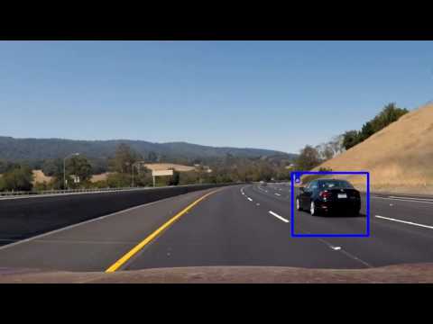
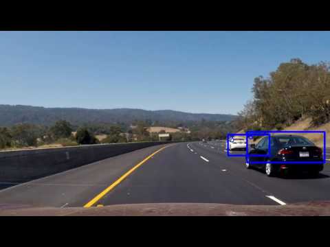
####2. Show some examples of test images to demonstrate how your pipeline is working. What did you do to optimize the performance of your classifier?

Ultimately I searched on three scales using YCrCb 2-channel (0 and 1) HOG features plus spatially (spatial size of 16x16) binned color in the feature vector. Some example images are given below.

####3. Convolutional Neural Network

Another classifier used in the project was a convolutional neural network. The model has two convolution layers as the following:

• 64 x 64 x 3 input
• 8 x 8 filter, with 6 depth, 4 x 4 stride, activation relu
• Dropout 0.5
• 8 x 8 filter, with 12 depth, 4 x 4 stride
• Flatten
• Dropout 0.5
• Activation relu
• Fully connected to 2 output
• Softmax

The convolutional neural network also trained with the complete data. 20% of the data was split as test set. The accuracy obtained was 0.9924 at epoch 50. The model is simple but it is faster than the SVM model with hog features.

Video Implementation

####1. Provide a link to your final video output. Your pipeline should perform reasonably well on the entire project video (somewhat wobbly or unstable bounding boxes are ok as long as you are identifying the vehicles most of the time with minimal false positives.)

Project video processed with Fast SVM model

Project video processed with Best SVM model

Project video processed with Fast SVM model

Project video processed with Fast SVM model

Project video processed with Fast SVM model

####2. Describe how (and identify where in your code) you implemented some kind of filter for false positives and some method for combining overlapping bounding boxes.

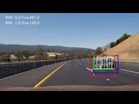
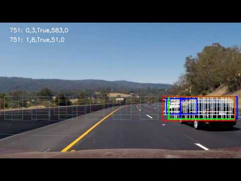
I recorded the positions of positive detections in each frame of the video. From the positive detections, I created a heatmap. If it was the first image of the pipeline or a single image, i thresholded that heatmap with 1. Otherwise, I combined the heatmaps of the previous image up to 5 images by summing the values. Then, I applied threshold to the combined heatmap by the number of heatmaps combined and the ratio 0.75. These thresholds were applied in the process_image function in the code cell 29. These values were used for the Fast model. For the Best SVM model, process_image_best function in the code cell 30, and for the CNN model, process_image_cnn function in the code cell 37 were used. I then used scipy.ndimage.measurements.label() to identify individual blobs in the heatmap. Then, for each blob, I compared the x and y values with the vehicles in the list. If a blob and a vehicle have an intersection, then the blob assumed to pair with that vehicle.

I constructed bounding boxes to cover the area of each vehicle in the vehicle list. The vehicle list was kept with Tracker class in the code cell 22. The vehicle class is in the code cell 20. The function draw_labeled_bboxes_reverse, located in the 25th code cell, takes image, labels and the tracker object as input parameters. When matching the blobs of labels with vehicles, if a label has an area of 1.5 times the area of the vehicle, it is assumed that the label is too big for the vehicle, and there is another vehicle associated with the same label. And the vehicle assumed to be hiding if the vehicle is completely on the inside of the label.

If a label is not associated with existing vehicles, then it is added as a new vehicle. A vehicle is considered to be reliable if it is detected more than or equal to 10 times.

If a vehicle is not detected for 5 (v_visible) times consecutively, it will not be shown. For reliable vehicles, the number of non-detected frames is increased by 15 (last_n). If a vehicle not detected 10 (remove_n) times, and it is removed from the list. For reliable vehicles, this number is doubled.

Here are six frames and their corresponding heatmaps:

Here is the output of scipy.ndimage.measurements.label() on the integrated heatmap from all six frames:

Here the resulting bounding boxes are drawn onto the last frame in the series:

---

###Discussion

####1. Briefly discuss any problems / issues you faced in your implementation of this project. Where will your pipeline likely fail? What could you do to make it more robust?

I have spent a significant amount of time to find parameters to extract features that should enable the classifier run in near time and have an accuracy value greater than 0.99, which I believe to be necessary to make the pipeline reliable. However, I was not able to find such parameters. The fastest parameters I can come up with processed the project video a rate of 3 frames per second. I have also tried a faster model which has a processing rate greater than 3.5 frames per second; however, there were false positives. It requires more time to find a faster model that is also reliable.

I also tried to train a convolutional neural network with the same goal. I did not spend much time on it, but it seemed more promising.

This pipeline assumes the camera position will be stayed fix and searches only the windows for this camera position. I tried it with the challenge video from the Advanced Lane Finding project, it was able to detect vehicles, however, there were false positives that may be dangerous.

Developing models other parameters, especially the parameters obtained from the comparison 7, can be tried as future work. In addition, other ensembles such as ensembling three hog channels or ensembling hog channels from different color spaces may perform better. In order to increase processing speed, all of the training data may be resized to a lower resolution. However, working with convolutional neural networks probably lead to better results.

Process times and the models are given in the table below:

Model	Process Time	FPS	Accuracy
Fast	7:15	2.80	99.11%
Best	13:13	1.62	99.34%
CNN	1:50	11.40	99.24%

The tracking pipeline was optimized for the Fast SVM model, therefore, the performance of other models can be improved.