Add plot.violin() #335

JS3xton · 2020-05-24T22:17:02Z

Add plot.violin(), which easily and flexibly illustrates violin plots from flow cytometry data.

Closes #332.

Still TODO: create tutorial images and update image links in /doc/python_tutorial/plot.rst.

Wishlist:

Support logicle scale. (y-axis only?)
Add density parameter? (like normed_area parameter of plot.hist1d)
Support pd.Series and pd.Dataframe inputs? (probably better left to Add support for pandas DataFrames #76)

Testing:

In both Python 3.8 + Anaconda 2020.02 and Python 2.7 + Anaconda 4.4.0:

All unit tests pass.
The updated example analysis scripts run without error (analyze_no_mef.py, analyze_mef.py, and analyze_excel_ui.py in /examples).
The plot violin tutorial commands run without error (in /doc/python_tutorial/plot.rst).

Thoughts on some failure modes:

Supporting the channel parameter, which all plot functions offer, was a bit tricky given how flexible my original code was to different inputs. If plot.violin() is used correctly, it works as described. There are some potentially common failure modes, though:

plot.violin(fcs_data) (without channel) will attempt to plot each row of fcs_data as a violin. This happens because plot.violin() understands fcs_data to be a sequence of 1D sequences (which it technically is). This can be bad for fcs_data with many rows.
plot.violin([fcs_data1,fcs_data2,fcs_data3]) (again without channel) will concatenate all channels for each fcs_data and attempt to plot them, which usually fails trying to calculate log(0). This happens because the input is understood to be a sequence of 1D arrays, and each 1D array is iterated over using the .flat numpy iterator feature.

I chose not to address these failure modes, but I still wanted to point them out.

matplotlib was previously imported as "mpl" in plot_violin code. In FlowCal, matplotlib is not imported under this alias. This commit corrects "mpl" references to "matplotlib".

-Using a pd.Series for `positions` with a 0 position would fail because using `0 in positions` would check if 0 was in the index, not the positions. -x ticks would not be properly labeled under some circumstances because the plot was not properly drawn initially.

Fix plot.violin bug where channel was not extracted from zero, min, or max data.

-Made custom tick locators and formatters aware of min, max, and zero violins. -Exposed min, max, and zero violin tick labels for user to specify if so desired.

JS3xton · 2020-05-24T22:55:46Z

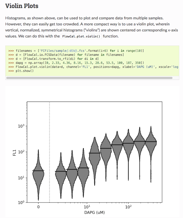
Example and tutorial plots (as of `90fed69`):

dose_response_violin.png generated by /examples/analyze_excel_ui.py:

From the tutorial:

FlowCal.plot.violin(data=d, channel='FL1', positions=iptg, xlabel='IPTG (uM)')

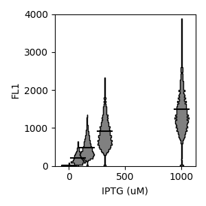
FlowCal.plot.violin(data=d, channel='FL1', positions=iptg, xlabel='IPTG (uM)', yscale='linear', ylim=(0,4000))

FlowCal.plot.violin(data=d, channel='FL1', positions=iptg, xlabel='IPTG (uM)', xscale='log')

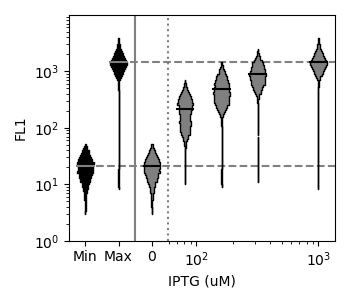
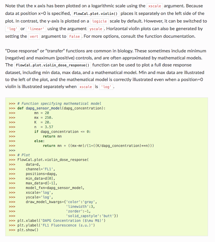
FlowCal.plot.violin(data=d,
                    min_data=d[0],
                    max_data=d[-1],
                    channel='FL1',
                    positions=iptg,
                    xlabel='IPTG (uM)',
                    xscale='log',
                    violin_kwargs={'data':{'facecolor':'gray', 'edgecolor':'black'},
                                   'min' :{'facecolor':'black','edgecolor':'black'},
                                   'max' :{'facecolor':'black','edgecolor':'black'}},
                    draw_summary_stat_kwargs={'data':{'color':'black'},
                                              'min' :{'color':'gray'},
                                              'max' :{'color':'gray'}})

def iptg_hill_model(iptg_concentration):
    mn = 20.
    mx = 1700.
    K  = 300.
    n  = 1.5
    if iptg_concentration <= 0:
        return mn
    else:
        return mn + ((mx-mn)/(1+((K/iptg_concentration)**n)))

FlowCal.plot.violin(data=d,
                    min_data=d[0],
                    max_data=d[-1],
                    channel='FL1',
                    positions=iptg,
                    xlabel='IPTG (uM)',
                    xscale='log',
                    violin_kwargs={'data':{'facecolor':'gray', 'edgecolor':'black'},
                                   'min' :{'facecolor':'black','edgecolor':'black'},
                                   'max' :{'facecolor':'black','edgecolor':'black'}},
                    draw_summary_stat_kwargs={'data':{'color':'black'},
                                              'min' :{'color':'gray'},
                                              'max' :{'color':'gray'}},
                    draw_model=True,
                    draw_model_fxn=iptg_hill_model,
                    draw_model_kwargs={'color':'gray',
                                       'linewidth':3,
                                       'zorder':-1,
                                       'solid_capstyle':'butt'},
                    data_xlim=(2e1,2e3))

castillohair · 2020-06-13T20:56:43Z

Cool! I'm excited to get this out.

I'm gonna start with some high-level questions. I'll get to specific code questions later.

Why is the default color gray, instead of being taken from the color cycle?
I'm not sure how I feel about the automatic inclusion of a violin for position zero when the x axis is logarithmic. Normally in matplotlib, when the axis is logarithmic, any points corresponding to position zero are just not plotted. The behavior of your function more closely resembles symlog.
In this section of your last example:

FlowCal.plot.violin(data=d,
                    min_data=d[0],
                    max_data=d[-1],

It seems that the FCSData objects passed to min_data and max_data also have to be passed to data. Is this correct? If it is, it is super confusing.

~~Can the y axis be logicle?~~ missed that part sry
Is there currently an easy option to increase or decrease the number of bins in the violins? in each violin independently?
I like that the code examples have been modified to include violin plots. I think we should make it as comparable as possible to the existing line plot (color, axis scales, figure size, etc).
What happens if, instead of plotting a continuous line using your draw_model parameters, I want to do that by calling plt.plot() after? Would this work?

JS3xton · 2020-06-14T18:50:22Z

Why is the default color gray, instead of being taken from the color cycle?

Just personal preference. I found it helpful to outline the violins with black lines. I also found it helpful to differentiate controls (min and max) with a separate face color. Black and gray seemed like natural grayscale colors that would look clean in a publication. I almost always ended up specifying a new color manually, though.

I'm not sure how I feel about the automatic inclusion of a violin for position zero when the x axis is logarithmic. Normally in matplotlib, when the axis is logarithmic, any points corresponding to position zero are just not plotted. The behavior of your function more closely resembles symlog.

That was born out of practicality. I was frequently visualizing violins with log-spaced x-positions but also wanting to show a zero violin.

We could make it less automatic by only illustrating the zero violin when specified via logx_zero_data instead of also looking for it in data.

I might also be open to supporting a symlog x-axis. I just wasn't prepared to implement it.

It seems that the FCSData objects passed to min_data and max_data also have to be passed to data. Is this correct? If it is, it is super confusing.

No, min_data and max_data don't have to be passed to data. That was me working around the fact that the sample files don't contain min or max control data, so I just used the available low and high concentrations. This is mentioned in the text of the new tutorial, where those examples would be shown:

Data for minimum and maximum controls can also be separately illustrated via the ``min_data`` and ``max_data`` parameters (here, we use the low and high IPTG concentrations).

Is there currently an easy option to increase or decrease the number of bins in the violins? in each violin independently?

Yes, the num_y_bins and y_bin_edges parameters can be used to control the number of bins. Separate calls to plot.violin would be required to control those on a per-violin basis, though.

I like that the code examples have been modified to include violin plots. I think we should make it as comparable as possible to the existing line plot (color, axis scales, figure size, etc).

That sounds like a good idea. I've made the violins look pretty, and I think the line plot looks kinda tacky, so I'd vote for updating the line plots. Specifically, it seems wider than it needs to be, and both axes are linear – I'd switch them to log to match the violin plot (or maybe symlog x-axis?).

What happens if, instead of plotting a continuous line using your draw_model parameters, I want to do that by calling plt.plot() after? Would this work?

Yes, you should absolutely still be able to use plt.plot() after plot.violin. The only issue is the user probably doesn't know where the min, max, and zero-violin boundaries are. Using draw_model will take care of properly terminating your line at the boundary. It will also illustrate the zero value as a flat line in the zero-violin portion of the plot, if appropriate. If min, max, and zero violins are not separately illustrated, though, there's no benefit to using draw_model.

castillohair · 2020-06-15T02:22:56Z

There are two extreme ways in which you can construct a plotting function. One is the "minimalist" approach, where the function does only the one thing that makes it "special" (e.g. making a scatter plot where the dots are colored according to density) but leave everything else to matplotlib (axis, labels, limits, etc.). This makes our function behave pretty much like any native matplotlib function. The other is the "rigid" approach, where the function sets the secondary properties in a way that further changes after the function call, such as colors or axis scales, are either impossible or they break the resulting plot. In general, I think been closer to the former is better because it makes the functions more intuitive to use (at least to a person already familiar with matplotlib), but this may get more difficult as the plotting function becomes more complex and/or specialized.

I think we have previously done a decent job with FlowCal in making our plotting functions "minimalist", although this is not perfect (e.g. our functions have arguments such as "xaxis" and "saveas" which are not matplotlib standard). I have the impression that this violin function in its current form is more to the "rigid" end of the spectrum, and that comes from the fact that it is currently made to replace a "transfer function" plot (i.e. continuous x axis, making it easy to have a violin for x=0, making it easy to insert min/max violins). In other words, as it stands, this is not just a violin plot function, as you could envision other types (e.g. the one in Felix's paper that substitutes a bar plot).

Still, this is a terribly useful function, but I think we need to clearly define what we're trying to do:

If we want to do violin plots in general, I think we would need to make a "minimalist" version that could be easily integrated with, at minimum, transfer function and bar plots, and possibly anything else that we're forgetting. The x axis would depend on what type of plot is being made and would be under the control of matplotlib. The y axis will be under control of FlowCal, and ideally would support all of the axis scales within, including logicle. More specialized functions would take this functionality to make a more specific type of plot (example name: violin_tf(), would do exactly what your function is currently doing).
Of course, we could just settle for making the specialized version you're presenting only. But if we do this, we might consider describing it as a "violin transfer function" plot. I think if we did this I would have an easier time accepting some of the idiosyncrasies such as automatic zero, min/max, color, etc.

Feel free to agree or disagree with whatever. My opinion on what changes, if any, this function needs is still being formed.

castillohair · 2020-06-15T02:24:43Z

Also apparently this branch has conflicts with develop. I would appreciate if you could fix those.

JS3xton · 2020-06-15T04:23:37Z

Yeah, this is a great point. I've also come over to the camp that "minimalist" is best, and I tried to write plot.violin to be minimalist. And as you say, it's not perfect – I added in the xlabel, ylabel, title, and savefig parameters to conform to our other plotting functions.

Now, you say you perceive plot.violin to be "rigid", but I would argue that it's actually very flexible. You're right that some of the advanced features (min, max, log-zero) can make the plot rigid, but if you don't use those, plot.violin will simply plot as many violins as you give it (down to a single one). So you can actually build a violin plot manually – one violin at a time – with repeated calls to plot.violin as it's currently written. Similarly, you should be able to use it with other transfer function or bar plots, as you say.

We could consider separating out the more advanced features to a separate function, but I initially lean against that because it actually seems less simple to me to have both a plot.violin function and a plot.violin_tf function. Having just plot.violin where 90% of the use cases don't use the advanced features seems fine to me. And if the documentation is good, the advanced features shouldn't confuse the user (that may still need some work? Maybe some simple examples in the docstring? Maybe adding an "Advanced Parameters" section instead of putting min_data, max_data, and log_zero_data front and center, which I admit was me being a little preachy and thinking "well everyone should specify these things..."). Additionally, you'd probably have to duplicate a nontrivial amount of code to keep the default parameters consistent between the two functions (a lot of the extra complexity in plot.violin is just calculating pretty-looking defaults). You might check out the _plot_violin() helper function, though, which is the bare-bones no-defaults function that actually draws a single violin.

The x axis would depend on what type of plot is being made and would be under the control of matplotlib.

Creating symmetrical violins requires knowing the scale of the x-axis, so xscale must be specified to plot.violin. You actually can change the x-scale with plt.xscale() after calling plot.violin, but the violins look distorted, as you might expect. You'd have to dynamically redraw the violins based on the x-scale to keep up with changes via plt.xscale(), and I don't think we should try and go down that rabbit hole.

Adding support for other types of x-scales might be worth investigating, though (symlog? logicle?).

The y axis will be under control of FlowCal, and ideally would support all of the axis scales within, including logicle.

Agreed. I wasn't comfortable enough with your implementation of logicle scaling to do it on this first pass, though.

Also apparently this branch has conflicts with develop. I would appreciate if you could fix those.

Yeah, I can resolve merge conflicts. I may wait until develop is more stable after some other things are resolved first, though.

FlowCal/plot.py

castillohair · 2020-07-04T19:42:37Z

FlowCal/plot.py

+        positions_length = len(positions)
+
+        if logx_zero_data is None:
+            logx_zero_data = zero_data


Maybe there needs to be a warning here if log_zero_data is not None? In this case, data[zero_idx] will be ignored, which may not be immediately obvious to the user.

Yeah, I think that's a good idea if we keep this behavior. The silent preference for log_zero_data over data[zero_idx] could otherwise be dubious.

You originally weren't sure about this automatic separation of the zero violin, though. I offered the alternative of ignoring data[zero_idx] if the x-axis is logarithmic, but we never resolved the issue.

castillohair · 2020-07-04T19:55:45Z

FlowCal/plot.py

+        Number of bins to bin population members into along the y-axis.
+        Ignored if `y_bin_edges` is specified.
+    y_bin_edges : sequence of scalars, sequence of sequence of scalars, or
+                  mapping to sequence of scalars, optional


Do we expect any mapping other than dictionaries? Dictionaries appear to be the only standard mapping in python. I would suggest simplifying the terminology to "dictionary".

Same with "sequence" -> "list", unless we're expecting an array, for which there is the "array_like" term. This would make it more consistent with the rest of Flowcal.plot.

I don't know what you mean by "expect". If robust, the function should work with any reasonable input. My nomenclature is intended to be as general as possible and is inspired by Python's Abstract Base Classes (ABCs), which include Sequence and Mapping. Moreover, the Sequence and Mapping ABCs are used pretty extensively throughout the code. So I guess you could say the code expects anything that is a Sequence or a Mapping.

More concretely, Sequence includes list and tuple, and Mapping includes dict and OrderedDict.

It appears ndarray doesn't quite make the cut for Sequence: numpy/numpy#2776, numpy/numpy#7315. This could actually be an issue in a few places (e.g. specifying upper_trim_fraction or lower_trim_fraction as an ndarray of floats); I didn't test ndarrays extensively.

And array_like can actually be quite vague: https://stackoverflow.com/a/40380014.

Ultimately, I wanted tuple to work as well as list and ndarray anywhere I said "sequence". pd.Series and pd.DataFrame would also be nice, but I consider those the purview of #76.

I understand that you're trying to be general with these abstract classes, but these Sequence and Mapping names are not widespread and make the documentation more confusing than it needs to be. I didn't even know of their existence, and only knew where to look them up after seeing that they come from collections after looking at the code. Furthermore, these are not used anywhere else in FlowCal, and it is very inconsistent to have one single function that suddenly uses this nomenclature. I'd rather use list and dictionary and drop the theoretical compatibility with other Sequence and Mapping objects, and gain in terms of documentation readability.

Are you advocating for dumbing down the code? Or just the documentation?

Furthermore, these are not used anywhere else in FlowCal, and it is very inconsistent to have one single function that suddenly uses this nomenclature.

I agree here. Although I'd prefer improving the robustness everywhere else. There are several places where isinstance(..., list) is used, which unnecessarily prevents other sequence data structures (namely tuple). The documentation usually specifies list, at least, but it still feels unnecessarily restrictive. This would obviously have to be a separate issue, though.

We also appear to use numpy array and array_like interchangeably in some spots? Which is kinda confusing.

Are you advocating for dumbing down the code? Or just the documentation?

Just for the documentation and error messages. The code looks fine and is probably more robust as you said. We can claim we provide support for the basic data structures and silently provide support for the more general abstract classes.

Ahh, OK cool. Yeah, I can get behind that.

FlowCal/plot.py

castillohair · 2020-07-04T20:40:36Z

FlowCal/plot.py

+        violin's position, 'data'. Min, max, and zero kwargs can be specified
+        via the 'min', 'max', and 'logx_zero' keys, respectively. If
+        `violin_kwargs` is a sequence of mappings, min, max, and zero violins
+        cannot be used. Default = {'facecolor':'gray', 'edgecolor':'black'}.


This needs examples. It's a little hard to understand.

Agreed.

Several parameters behave similarly in this regard. I'm not sure if it's better to make separate examples for all of them or to reorganize the docstring and consolidate like parameters. E.g. adding a "Per-Violin Parameters" section and explaining the different ways they can be specified.

The problem with the "Per-Violin Parameters" idea is that I don't know how sphinx would parse it when generating the documentation. I'm OK with having examples for every parameter, even if that means that there is some repetition.

sphinx parses "Other Parameters" sections for many functions in the plot module. Is there any reason to believe a "Per-Violin Parameters" section (or an "Advanced Parameters" section for min_data, max_data, and log_zero_data, as discussed previously) would be treated any differently?

There is a documented "Other Parameters" section in the numpydoc specification.

castillohair · 2020-07-04T20:41:06Z

FlowCal/plot.py

+        and zero `draw_summary_stat_kwargs` can be specified via the 'min',
+        'max', and 'logx_zero' keys, respectively. If
+        `draw_summary_stat_kwargs` is a sequence of mappings, min, max, and
+        zero violins cannot be used. Default = {'color':'black'}.


This also needs examples.

see response above

castillohair · 2020-07-05T06:37:28Z

FlowCal/plot.py

+                     draw_summary_stat_fxn=draw_summary_stat_fxn,
+                     draw_summary_stat_kwargs=v_draw_summary_stat_kwargs)
+
+        if draw_model:


Why is this inside the for idx in range(data_length):? Does this mean that the model plot is made every time a new violin is plotted?

Hmm, good catch. Yeah, that should probably be unindented once.

castillohair · 2020-07-05T08:22:36Z

Having read the code, I still think these should be made into two functions. The mere existence of the advanced transfer function-specific parameters complicates how parameters are interpreted, which makes the documentation really hard to follow. For example, violin_kwargs currently can be one dictionary with kwargs, or a list of dictionaries that correspond to each data point, or a dictionary with keys data, min, and max and values that are kwarg dictionaries, and maybe other things that I'm missing. For a person that only wants to plot violins at certain positions, this can get overwhelming. And there are many parameters with similar behavior. You could make the documentation simpler, but you would have to hide or bury more and more information about the advanced features. Thus, there will be a tradeoff between making the function and its documentation simple and showcasing the advanced tf-specific features. But we can actually have both things if we make a function that is simple to use for the basic use case, and another where the tf-specific features are at the forefront.

Therefore, I think these should be split in the following way:

violin(), which would plot violins from data at positions. violin_kwargs and other similar parameters can only be a dictionary with kwargs or a list of dictionaries, each corresponding to an entry in data. In an ideal world, this function would support symlog, which would take care of plotting at position zero in a log scale. However, if this is too complicated, violin() should retain the ability to plot at position zero that you coded. But I think this should be done transparently - taking the violin for position zero from data automatically, and eliminating the parameter logx_zero_data.
violin_tf() (or some other name), which would call violin() to plot the data, and then plot the min/max violins and the "model" function. violin_kwargs here would only be allowed to be a dictionary with kwargs, or a dictionary with keys data, min, and max and kwarg dictionaries as values.

Also, I like that _plot_violin() is its own function but I think it should be renamed to something like _plot_single_violin(). Looking at the code, it seems to me that this is the only function that needs to be modified for logicle on the y axis to work. I can try to get this working.

JS3xton · 2020-07-05T18:56:40Z

(sorry, I just saw your last summary comment)

I think I'd be amenable to most of what you're suggesting.

violin(), which would plot violins from data at positions. violin_kwargs and other similar parameters can only be a dictionary with kwargs or a list of dictionaries, each corresponding to an entry in data. In an ideal world, this function would support symlog, which would take care of plotting at position zero in a log scale. However, if this is too complicated, violin() should retain the ability to plot at position zero that you coded. But I think this should be done transparently - taking the violin for position zero from data automatically, and eliminating the parameter logx_zero_data.

This sounds good to me. Nice and simple.

I'm still not sure how best to handle data at position zero, but I think that'll become clearer after we look into symlog. (I don't think symlog is an exact replacement for the current behavior, but it's a good option to consider supporting.) Setting zero aside transparently and eliminating logx_zero_data sounds good to me.

violin_tf() (or some other name), which would call violin() to plot the data, and then plot the min/max violins and the "model" function. violin_kwargs here would only be allowed to be a dictionary with kwargs, or a dictionary with keys data, min, and max and kwarg dictionaries as values.

A better name would help me digest this one. tf is obscure and too specific (plots other than transfer functions can also be illustrated this way). Perhaps violin_with_controls or violin_and_controls. Or violin_with_controls_and_model...

Regarding violin_kwargs, it might be better to just add min_violin_kwargs and max_violin_kwargs parameters. That way we can keep violin_kwargs consistent with violin(), allowing users to more seamlessly transition between violin() to violin_tf().

Also, I like that _plot_violin() is its own function but I think it should be renamed to something like _plot_single_violin(). Looking at the code, it seems to me that this is the only function that needs to be modified for logicle on the y axis to work. I can try to get this working.

That name change sounds good to me.

The yscale is currently set outside of _plot_violin(), so it may not even need to change. And you'd probably also need to modify the y_bin_edges defaults to add a Logicle option.

castillohair · 2020-07-05T23:18:19Z

A better name would help me digest this one. tf is obscure and too specific (plots other than transfer functions can also be illustrated this way). Perhaps violin_with_controls or violin_and_controls. Or violin_with_controls_and_model...

In old-school biology papers, these "transfer functions" are usually called "dose response curves" (e.g. https://academic.oup.com/nar/article/25/6/1203/1197243). I say we fully embrace the function's intended application and use something like violin_dose_response() instead of something long like violin_with_controls_and_model().

Regarding violin_kwargs, it might be better to just add min_violin_kwargs and max_violin_kwargs parameters. That way we can keep violin_kwargs consistent with violin(), allowing users to more seamlessly transition between violin() to violin_tf().

Sounds good to me.

JS3xton · 2020-07-08T20:15:09Z

A better name would help me digest this one. tf is obscure and too specific (plots other than transfer functions can also be illustrated this way). Perhaps violin_with_controls or violin_and_controls. Or violin_with_controls_and_model...

In old-school biology papers, these "transfer functions" are usually called "dose response curves" (e.g. https://academic.oup.com/nar/article/25/6/1203/1197243). I say we fully embrace the function's intended application and use something like violin_dose_response() instead of something long like violin_with_controls_and_model().

Hmm, I definitely like violin_dose_response() better than violin_tf(). violin_dose_response() still doesn't quite sit right for me (dose responses can still be plotted with plot.violin(), for example), but I don't have a better alternative, so I think we go with that for now.

castillohair · 2020-07-08T21:10:27Z

As we discussed, we should also change the example files with one of the datasets in your paper since they illustrate the features of violin_dose_response() best.

We would need to change the example FCS files of course, and change the Excel file and the .py scripts.
The tutorial in the documentation will need some minor changes. I can get onto this once everything else is done.
Hopefully we don't have any unit tests that depend on the example files. If we do, they will need to be adjusted.

JS3xton · 2020-10-07T02:05:49Z

bc98686 adds a vert parameter to plot.violin(), which allows violins to be plotted horizontally.

Support for horizontal violins was added symmetrically, so position=0 violins are separately illustrated for both vertical and horizontal violin plots when the position axis is logarithmic. plot.violin_dose_response() still only supports vertical violins. Some plot.violin() and plot.violin_dose_response() parameters were renamed to remove references to axes (e.g., y_bin_edges -> bin_edges).

Unit tests still pass in Python 3.8 + Anaconda 2020.07 and Python 2.7 + Anaconda 5.2.0. The example analysis scripts still run without error. Updated versions of the tutorial code also ran without error.

Additional code used for testing:

plot.violin() stress test code

import FlowCal
import numpy as np
import matplotlib.pyplot as plt
filenames = ['FCFiles/Data{:03d}.fcs'.format(i) for i in range(1,5+1)]
d = [FlowCal.io.FCSData(filename) for filename in filenames]
d = [FlowCal.transform.to_rfi(di) for di in d]
iptg = [0, 81, 161, 318, 1000]

figsize=(3,2.5)

plt.figure(figsize=figsize)
FlowCal.plot.violin(data=d, channel='FL1', positions=iptg, xlabel='IPTG (uM)')



plt.figure(figsize=figsize)
FlowCal.plot.violin(data=d, channel='FL1', positions=iptg, xlabel='IPTG (uM)', yscale='linear', ylim=(0,4000), bin_edges=np.linspace(0,4000,101), lower_trim_fraction=0)

plt.figure(figsize=figsize)
FlowCal.plot.violin(data=d, channel='FL1', positions=iptg, xlabel='IPTG (uM)', yscale='linear', ylim=(0,4000), bin_edges=np.linspace(0,4000,101), density=True, lower_trim_fraction=0)

plt.figure(figsize=figsize)
FlowCal.plot.violin(data=d, channel='FL1', positions=iptg, xlabel='IPTG (uM)', yscale='linear', ylim=(0,4000), bin_edges=np.logspace(0,4,101), lower_trim_fraction=0)

plt.figure(figsize=figsize)
FlowCal.plot.violin(data=d, channel='FL1', positions=iptg, xlabel='IPTG (uM)', yscale='linear', ylim=(0,4000), bin_edges=np.logspace(0,4,101), density=True, lower_trim_fraction=0)


plt.figure(figsize=figsize)
FlowCal.plot.violin(data=d, channel='FL1', positions=iptg, xlabel='IPTG (uM)', yscale='log', bin_edges=np.linspace(1,4000,201), lower_trim_fraction=0)

plt.figure(figsize=figsize)
FlowCal.plot.violin(data=d, channel='FL1', positions=iptg, xlabel='IPTG (uM)', yscale='log', bin_edges=np.linspace(1,4000,201), density=True, lower_trim_fraction=0)

plt.figure(figsize=figsize)
FlowCal.plot.violin(data=d, channel='FL1', positions=iptg, xlabel='IPTG (uM)', yscale='log', bin_edges=np.logspace(0,4,101), lower_trim_fraction=0)

plt.figure(figsize=figsize)
FlowCal.plot.violin(data=d, channel='FL1', positions=iptg, xlabel='IPTG (uM)', yscale='log', bin_edges=np.logspace(0,4,101), density=True, lower_trim_fraction=0)



plt.figure(figsize=figsize)
FlowCal.plot.violin(data=d, channel='FL1', positions=iptg, xlabel='IPTG (uM)', xscale='log')

plt.figure(figsize=figsize)
FlowCal.plot.violin(data=d[1:], channel='FL1', positions=iptg[1:], xlabel='IPTG (uM)', xscale='log')

plt.figure(figsize=figsize)
FlowCal.plot.violin(
data=d,
channel='FL1',
positions=iptg,
xlabel='IPTG (uM)',
xscale='log',
violin_width=0.5,
ylim=(1e0,1e4),
xlim=(1e1,1e4),
num_bins=30)

plt.figure(figsize=figsize)
FlowCal.plot.violin(
data=d,
channel='FL1',
positions=iptg,
xlabel='IPTG (uM)',
xscale='log',
violin_width=0.5,
ylim=(1e0,1e4),
xlim=(1e1,1e4),
bin_edges=np.logspace(0,4,30))

plt.figure(figsize=figsize)
FlowCal.plot.violin(
data=d,
channel='FL1',
positions=iptg,
xlabel='IPTG (uM)',
xscale='log',
violin_width=0.5,
ylim=(1e0,1e4),
xlim=(1e1,1e4),
bin_edges=np.logspace(0,4,30),
upper_trim_fraction=0.1,
lower_trim_fraction=0.05)

plt.figure(figsize=figsize)
FlowCal.plot.violin(
data=d,
channel='FL1',
positions=iptg,
xlabel='IPTG (uM)',
xscale='log',
violin_width_to_span_fraction=0.025,
ylim=(1e0,1e4),
xlim=(1e1,1e4),
bin_edges=np.logspace(0,4,30),
upper_trim_fraction=0.1,
lower_trim_fraction=0.05)


plt.figure(figsize=figsize)
FlowCal.plot.violin(
data=d,
channel='FL1',
positions=iptg,
xlabel='IPTG (uM)',
xscale='log',
violin_width=0.5,
ylim=(1e0,1e4),
xlim=(1e1,1e4),
bin_edges=np.logspace(0,4,30),
upper_trim_fraction=0.1,
lower_trim_fraction=0.05,
violin_kwargs={'facecolor':'red', 'edgecolor':'blue'})

plt.figure(figsize=figsize)
FlowCal.plot.violin(
data=d,
channel='FL1',
positions=iptg,
xlabel='IPTG (uM)',
xscale='log',
violin_width=0.5,
ylim=(1e0,1e4),
xlim=(1e1,1e4),
bin_edges=np.logspace(0,4,30),
upper_trim_fraction=0.1,
lower_trim_fraction=0.05,
violin_kwargs={'facecolor':'red', 'edgecolor':'blue'},
draw_summary_stat=False)

plt.figure(figsize=figsize)
FlowCal.plot.violin(
data=d,
channel='FL1',
positions=iptg,
xlabel='IPTG (uM)',
xscale='log',
violin_width=0.5,
ylim=(1e0,1e4),
xlim=(1e1,1e4),
bin_edges=np.logspace(0,4,30),
upper_trim_fraction=0.1,
lower_trim_fraction=0.05,
violin_kwargs={'facecolor':'red', 'edgecolor':'blue'},
draw_summary_stat_fxn=np.median,
draw_summary_stat_kwargs={'color':'green'})


plt.figure(figsize=figsize)
FlowCal.plot.violin(
data=d,
channel='FL1',
positions=iptg,
xlabel='IPTG (uM)',
xscale='log',
violin_width=0.5,
ylim=(1e0,1e4),
xlim=(1e1,1e4),
bin_edges=np.logspace(0,4,30),
upper_trim_fraction=0.1,
lower_trim_fraction=0.05,
violin_kwargs={'facecolor':'red', 'edgecolor':'blue'},
draw_summary_stat_fxn=np.median,
draw_summary_stat_kwargs={'color':'green'},
log_zero_tick_label='test')

plt.figure(figsize=figsize)
FlowCal.plot.violin(
data=d,
channel='FL1',
positions=iptg,
xlabel='IPTG (uM)',
xscale='log',
violin_width=0.5,
ylim=(1e0,1e4),
xlim=(1e1,1e4),
bin_edges=np.logspace(0,4,30),
upper_trim_fraction=0.1,
lower_trim_fraction=0.05,
violin_kwargs={'facecolor':'red', 'edgecolor':'blue'},
draw_summary_stat_fxn=np.median,
draw_summary_stat_kwargs={'color':'green'},
log_zero_tick_label='test',
draw_log_zero_divider_kwargs={'color':'purple'})



plt.figure(figsize=figsize)
FlowCal.plot.violin(
data=d,
channel='FL1',
positions=iptg,
xlabel='IPTG (uM)',
xscale='log',
violin_width=0.5,
ylim=(1e0,1e4),
xlim=(1e1,1e4),
bin_edges=[np.logspace(0,4,30),
           np.logspace(0,4,200),
           np.logspace(0,4,20),
           np.logspace(0,4,200),
           np.logspace(0,4,30)],
upper_trim_fraction=[0.1, 0.25, 0.01, 0.1, 0.01],
lower_trim_fraction=[0.25, 0.01, 0.1, 0.05, 0.1],
violin_kwargs=[{'facecolor':'red', 'edgecolor':'purple'},
               {'facecolor':'orange', 'edgecolor':'blue'},
               {'facecolor':'yellow', 'edgecolor':'green'},
               {'facecolor':'green', 'edgecolor':'yellow'},
               {'facecolor':'blue', 'edgecolor':'orange'}],
draw_summary_stat_fxn=np.median,
draw_summary_stat_kwargs=[{'color':'blue'},
                          {'color':'black'},
                          {'color':'red'},
                          {'color':'blue'},
                          {'color':'white'},],
log_zero_tick_label='test',
draw_log_zero_divider_kwargs={'color':'purple'})

###
# vert
###

figsize=(2,2)

plt.figure(figsize=figsize)
FlowCal.plot.violin(data=d, channel='FL1', positions=iptg, ylabel='IPTG (uM)', vert=False)



plt.figure(figsize=figsize)
FlowCal.plot.violin(data=d, channel='FL1', positions=iptg, ylabel='IPTG (uM)', xscale='linear', xlim=(0,4000), bin_edges=np.linspace(0,4000,101), lower_trim_fraction=0, vert=False)

plt.figure(figsize=figsize)
FlowCal.plot.violin(data=d, channel='FL1', positions=iptg, ylabel='IPTG (uM)', xscale='linear', xlim=(0,4000), bin_edges=np.linspace(0,4000,101), density=True, lower_trim_fraction=0, vert=False)

plt.figure(figsize=figsize)
FlowCal.plot.violin(data=d, channel='FL1', positions=iptg, ylabel='IPTG (uM)', xscale='linear', xlim=(0,4000), bin_edges=np.logspace(0,4,101), lower_trim_fraction=0, vert=False)

plt.figure(figsize=figsize)
FlowCal.plot.violin(data=d, channel='FL1', positions=iptg, ylabel='IPTG (uM)', xscale='linear', xlim=(0,4000), bin_edges=np.logspace(0,4,101), density=True, lower_trim_fraction=0, vert=False)


plt.figure(figsize=figsize)
FlowCal.plot.violin(data=d, channel='FL1', positions=iptg, ylabel='IPTG (uM)', xscale='log', bin_edges=np.linspace(1,4000,201), lower_trim_fraction=0, vert=False)

plt.figure(figsize=figsize)
FlowCal.plot.violin(data=d, channel='FL1', positions=iptg, ylabel='IPTG (uM)', xscale='log', bin_edges=np.linspace(1,4000,201), density=True, lower_trim_fraction=0, vert=False)

plt.figure(figsize=figsize)
FlowCal.plot.violin(data=d, channel='FL1', positions=iptg, ylabel='IPTG (uM)', xscale='log', bin_edges=np.logspace(0,4,101), lower_trim_fraction=0, vert=False)

plt.figure(figsize=figsize)
FlowCal.plot.violin(data=d, channel='FL1', positions=iptg, ylabel='IPTG (uM)', xscale='log', bin_edges=np.logspace(0,4,101), density=True, lower_trim_fraction=0, vert=False)



plt.figure(figsize=figsize)
FlowCal.plot.violin(data=d, channel='FL1', positions=iptg, ylabel='IPTG (uM)', yscale='log', vert=False)

plt.figure(figsize=figsize)
FlowCal.plot.violin(data=d[1:], channel='FL1', positions=iptg[1:], ylabel='IPTG (uM)', yscale='log', vert=False)

plt.figure(figsize=figsize)
FlowCal.plot.violin(
data=d,
channel='FL1',
positions=iptg,
ylabel='IPTG (uM)',
yscale='log',
violin_width=0.5,
xlim=(1e0,1e4),
ylim=(1e1,1e4),
num_bins=30,
vert=False)

plt.figure(figsize=figsize)
FlowCal.plot.violin(
data=d,
channel='FL1',
positions=iptg,
ylabel='IPTG (uM)',
yscale='log',
violin_width=0.5,
xlim=(1e0,1e4),
ylim=(1e1,1e4),
bin_edges=np.logspace(0,4,30),
vert=False)

plt.figure(figsize=figsize)
FlowCal.plot.violin(
data=d,
channel='FL1',
positions=iptg,
ylabel='IPTG (uM)',
yscale='log',
violin_width=0.5,
xlim=(1e0,1e4),
ylim=(1e1,1e4),
bin_edges=np.logspace(0,4,30),
upper_trim_fraction=0.1,
lower_trim_fraction=0.05,
vert=False)

plt.figure(figsize=figsize)
FlowCal.plot.violin(
data=d,
channel='FL1',
positions=iptg,
ylabel='IPTG (uM)',
yscale='log',
violin_width_to_span_fraction=0.025,
xlim=(1e0,1e4),
ylim=(1e1,1e4),
bin_edges=np.logspace(0,4,30),
upper_trim_fraction=0.1,
lower_trim_fraction=0.05,
vert=False)


plt.figure(figsize=figsize)
FlowCal.plot.violin(
data=d,
channel='FL1',
positions=iptg,
ylabel='IPTG (uM)',
yscale='log',
violin_width=0.5,
xlim=(1e0,1e4),
ylim=(1e1,1e4),
bin_edges=np.logspace(0,4,30),
upper_trim_fraction=0.1,
lower_trim_fraction=0.05,
violin_kwargs={'facecolor':'red', 'edgecolor':'blue'},
vert=False)

plt.figure(figsize=figsize)
FlowCal.plot.violin(
data=d,
channel='FL1',
positions=iptg,
ylabel='IPTG (uM)',
yscale='log',
violin_width=0.5,
xlim=(1e0,1e4),
ylim=(1e1,1e4),
bin_edges=np.logspace(0,4,30),
upper_trim_fraction=0.1,
lower_trim_fraction=0.05,
violin_kwargs={'facecolor':'red', 'edgecolor':'blue'},
draw_summary_stat=False,
vert=False)

plt.figure(figsize=figsize)
FlowCal.plot.violin(
data=d,
channel='FL1',
positions=iptg,
ylabel='IPTG (uM)',
yscale='log',
violin_width=0.5,
xlim=(1e0,1e4),
ylim=(1e1,1e4),
bin_edges=np.logspace(0,4,30),
upper_trim_fraction=0.1,
lower_trim_fraction=0.05,
violin_kwargs={'facecolor':'red', 'edgecolor':'blue'},
draw_summary_stat_fxn=np.median,
draw_summary_stat_kwargs={'color':'green'},
vert=False)


plt.figure(figsize=figsize)
FlowCal.plot.violin(
data=d,
channel='FL1',
positions=iptg,
ylabel='IPTG (uM)',
yscale='log',
violin_width=0.5,
xlim=(1e0,1e4),
ylim=(1e1,1e4),
bin_edges=np.logspace(0,4,30),
upper_trim_fraction=0.1,
lower_trim_fraction=0.05,
violin_kwargs={'facecolor':'red', 'edgecolor':'blue'},
draw_summary_stat_fxn=np.median,
draw_summary_stat_kwargs={'color':'green'},
log_zero_tick_label='test',
vert=False)

plt.figure(figsize=figsize)
FlowCal.plot.violin(
data=d,
channel='FL1',
positions=iptg,
ylabel='IPTG (uM)',
yscale='log',
violin_width=0.5,
xlim=(1e0,1e4),
ylim=(1e1,1e4),
bin_edges=np.logspace(0,4,30),
upper_trim_fraction=0.1,
lower_trim_fraction=0.05,
violin_kwargs={'facecolor':'red', 'edgecolor':'blue'},
draw_summary_stat_fxn=np.median,
draw_summary_stat_kwargs={'color':'green'},
log_zero_tick_label='test',
draw_log_zero_divider_kwargs={'color':'purple'},
vert=False)



plt.figure(figsize=figsize)
FlowCal.plot.violin(
data=d,
channel='FL1',
positions=iptg,
ylabel='IPTG (uM)',
yscale='log',
violin_width=0.5,
xlim=(1e0,1e4),
ylim=(1e1,1e4),
bin_edges=[np.logspace(0,4,30),
           np.logspace(0,4,200),
           np.logspace(0,4,20),
           np.logspace(0,4,200),
           np.logspace(0,4,30)],
upper_trim_fraction=[0.1, 0.25, 0.01, 0.1, 0.01],
lower_trim_fraction=[0.25, 0.01, 0.1, 0.05, 0.1],
violin_kwargs=[{'facecolor':'red', 'edgecolor':'purple'},
               {'facecolor':'orange', 'edgecolor':'blue'},
               {'facecolor':'yellow', 'edgecolor':'green'},
               {'facecolor':'green', 'edgecolor':'yellow'},
               {'facecolor':'blue', 'edgecolor':'orange'}],
draw_summary_stat_fxn=np.median,
draw_summary_stat_kwargs=[{'color':'blue'},
                          {'color':'black'},
                          {'color':'red'},
                          {'color':'blue'},
                          {'color':'white'},],
log_zero_tick_label='test',
draw_log_zero_divider_kwargs={'color':'purple'},
vert=False)

plt.show()

plot.violin_dose_response() stress test code

import FlowCal
import numpy as np
import matplotlib.pyplot as plt
filenames = ['FCFiles/Data{:03d}.fcs'.format(i) for i in range(1,5+1)]
d = [FlowCal.io.FCSData(filename) for filename in filenames]
d = [FlowCal.transform.to_rfi(di) for di in d]
iptg = [0, 81, 161, 318, 1000]

figsize=(3,2.5)

plt.figure(figsize=figsize)
FlowCal.plot.violin_dose_response(data=d, channel='FL1', positions=iptg, xlabel='IPTG (uM)')





plt.figure(figsize=figsize)
FlowCal.plot.violin_dose_response(data=d, channel='FL1', positions=iptg, xlabel='IPTG (uM)', yscale='linear', ylim=(0,4000), bin_edges=np.linspace(0,4000,101), lower_trim_fraction=0)

plt.figure(figsize=figsize)
FlowCal.plot.violin_dose_response(data=d, channel='FL1', positions=iptg, xlabel='IPTG (uM)', yscale='linear', ylim=(0,4000), bin_edges=np.linspace(0,4000,101), density=True, lower_trim_fraction=0)

plt.figure(figsize=figsize)
FlowCal.plot.violin_dose_response(data=d, channel='FL1', positions=iptg, xlabel='IPTG (uM)', yscale='linear', ylim=(0,4000), bin_edges=np.logspace(0,4,101), lower_trim_fraction=0)

plt.figure(figsize=figsize)
FlowCal.plot.violin_dose_response(data=d, channel='FL1', positions=iptg, xlabel='IPTG (uM)', yscale='linear', ylim=(0,4000), bin_edges=np.logspace(0,4,101), density=True, lower_trim_fraction=0)


plt.figure(figsize=figsize)
FlowCal.plot.violin_dose_response(data=d, channel='FL1', positions=iptg, xlabel='IPTG (uM)', yscale='log', bin_edges=np.linspace(1,4000,201), lower_trim_fraction=0)

plt.figure(figsize=figsize)
FlowCal.plot.violin_dose_response(data=d, channel='FL1', positions=iptg, xlabel='IPTG (uM)', yscale='log', bin_edges=np.linspace(1,4000,201), density=True, lower_trim_fraction=0)

plt.figure(figsize=figsize)
FlowCal.plot.violin_dose_response(data=d, channel='FL1', positions=iptg, xlabel='IPTG (uM)', yscale='log', bin_edges=np.logspace(0,4,101), lower_trim_fraction=0)

plt.figure(figsize=figsize)
FlowCal.plot.violin_dose_response(data=d, channel='FL1', positions=iptg, xlabel='IPTG (uM)', yscale='log', bin_edges=np.logspace(0,4,101), density=True, lower_trim_fraction=0)







plt.figure(figsize=figsize)
FlowCal.plot.violin_dose_response(data=d, channel='FL1', positions=iptg, xlabel='IPTG (uM)', xscale='log')

plt.figure(figsize=figsize)
FlowCal.plot.violin_dose_response(data=d[1:], channel='FL1', positions=iptg[1:], xlabel='IPTG (uM)', xscale='log')

plt.figure(figsize=figsize)
FlowCal.plot.violin_dose_response(
data=d,
channel='FL1',
positions=iptg,
xlabel='IPTG (uM)',
xscale='log',
violin_width=0.5,
ylim=(1e0,1e4),
xlim=(1e1,1e4),
num_bins=30)

plt.figure(figsize=figsize)
FlowCal.plot.violin_dose_response(
data=d,
channel='FL1',
positions=iptg,
xlabel='IPTG (uM)',
xscale='log',
violin_width=0.5,
ylim=(1e0,1e4),
xlim=(1e1,1e4),
bin_edges=np.logspace(0,4,30))

plt.figure(figsize=figsize)
FlowCal.plot.violin_dose_response(
data=d,
channel='FL1',
positions=iptg,
xlabel='IPTG (uM)',
xscale='log',
violin_width=0.5,
ylim=(1e0,1e4),
xlim=(1e1,1e4),
bin_edges=np.logspace(0,4,30),
upper_trim_fraction=0.1,
lower_trim_fraction=0.05)

plt.figure(figsize=figsize)
FlowCal.plot.violin_dose_response(
data=d,
channel='FL1',
positions=iptg,
xlabel='IPTG (uM)',
xscale='log',
violin_width_to_span_fraction=0.025,
ylim=(1e0,1e4),
xlim=(1e1,1e4),
bin_edges=np.logspace(0,4,30),
upper_trim_fraction=0.1,
lower_trim_fraction=0.05)


plt.figure(figsize=figsize)
FlowCal.plot.violin_dose_response(
data=d,
channel='FL1',
positions=iptg,
xlabel='IPTG (uM)',
xscale='log',
violin_width=0.5,
ylim=(1e0,1e4),
xlim=(1e1,1e4),
bin_edges=np.logspace(0,4,30),
upper_trim_fraction=0.1,
lower_trim_fraction=0.05,
violin_kwargs={'facecolor':'red', 'edgecolor':'blue'})

plt.figure(figsize=figsize)
FlowCal.plot.violin_dose_response(
data=d,
channel='FL1',
positions=iptg,
xlabel='IPTG (uM)',
xscale='log',
violin_width=0.5,
ylim=(1e0,1e4),
xlim=(1e1,1e4),
bin_edges=np.logspace(0,4,30),
upper_trim_fraction=0.1,
lower_trim_fraction=0.05,
violin_kwargs={'facecolor':'red', 'edgecolor':'blue'},
draw_summary_stat=False)

plt.figure(figsize=figsize)
FlowCal.plot.violin_dose_response(
data=d,
channel='FL1',
positions=iptg,
xlabel='IPTG (uM)',
xscale='log',
violin_width=0.5,
ylim=(1e0,1e4),
xlim=(1e1,1e4),
bin_edges=np.logspace(0,4,30),
upper_trim_fraction=0.1,
lower_trim_fraction=0.05,
violin_kwargs={'facecolor':'red', 'edgecolor':'blue'},
draw_summary_stat_fxn=np.median,
draw_summary_stat_kwargs={'color':'green'})


plt.figure(figsize=figsize)
FlowCal.plot.violin_dose_response(
data=d,
channel='FL1',
positions=iptg,
xlabel='IPTG (uM)',
xscale='log',
violin_width=0.5,
ylim=(1e0,1e4),
xlim=(1e1,1e4),
bin_edges=np.logspace(0,4,30),
upper_trim_fraction=0.1,
lower_trim_fraction=0.05,
violin_kwargs={'facecolor':'red', 'edgecolor':'blue'},
draw_summary_stat_fxn=np.median,
draw_summary_stat_kwargs={'color':'green'},
log_zero_tick_label='test')

plt.figure(figsize=figsize)
FlowCal.plot.violin_dose_response(
data=d,
channel='FL1',
positions=iptg,
xlabel='IPTG (uM)',
xscale='log',
violin_width=0.5,
ylim=(1e0,1e4),
xlim=(1e1,1e4),
bin_edges=np.logspace(0,4,30),
upper_trim_fraction=0.1,
lower_trim_fraction=0.05,
violin_kwargs={'facecolor':'red', 'edgecolor':'blue'},
draw_summary_stat_fxn=np.median,
draw_summary_stat_kwargs={'color':'green'},
log_zero_tick_label='test',
draw_log_zero_divider_kwargs={'color':'purple'})



plt.figure(figsize=figsize)
FlowCal.plot.violin_dose_response(
data=d,
channel='FL1',
positions=iptg,
xlabel='IPTG (uM)',
xscale='log',
violin_width=0.5,
ylim=(1e0,1e4),
xlim=(1e1,1e4),
bin_edges=[np.logspace(0,4,30),
           np.logspace(0,4,200),
           np.logspace(0,4,20),
           np.logspace(0,4,200),
           np.logspace(0,4,30)],
upper_trim_fraction=[0.1, 0.25, 0.01, 0.1, 0.01],
lower_trim_fraction=[0.25, 0.01, 0.1, 0.05, 0.1],
violin_kwargs=[{'facecolor':'red', 'edgecolor':'purple'},
               {'facecolor':'orange', 'edgecolor':'blue'},
               {'facecolor':'yellow', 'edgecolor':'green'},
               {'facecolor':'green', 'edgecolor':'yellow'},
               {'facecolor':'blue', 'edgecolor':'orange'}],
draw_summary_stat_fxn=np.median,
draw_summary_stat_kwargs=[{'color':'blue'},
                          {'color':'black'},
                          {'color':'red'},
                          {'color':'blue'},
                          {'color':'white'},],
log_zero_tick_label='test',
draw_log_zero_divider_kwargs={'color':'purple'})




def iptg_hill_model(iptg_concentration):
   mn = 20.
   mx = 1700.
   K  = 300.
   n  = 1.5
   if iptg_concentration <= 0:
       return mn
   else:
       return mn + ((mx-mn)/(1+((K/iptg_concentration)**n)))


plt.figure(figsize=figsize)
FlowCal.plot.violin_dose_response(
data=d,
model_fxn=iptg_hill_model,
channel='FL1',
positions=iptg,
xlabel='IPTG (uM)',
xscale='log',
violin_width=0.5,
ylim=(1e0,1e4),
xlim=(1e1,1e4),
bin_edges=[np.logspace(0,4,30),
           np.logspace(0,4,200),
           np.logspace(0,4,20),
           np.logspace(0,4,200),
           np.logspace(0,4,30)],
upper_trim_fraction=[0.1, 0.25, 0.01, 0.1, 0.01],
lower_trim_fraction=[0.25, 0.01, 0.1, 0.05, 0.1],
violin_kwargs=[{'facecolor':'red', 'edgecolor':'purple'},
               {'facecolor':'orange', 'edgecolor':'blue'},
               {'facecolor':'yellow', 'edgecolor':'green'},
               {'facecolor':'green', 'edgecolor':'yellow'},
               {'facecolor':'blue', 'edgecolor':'orange'}],
draw_summary_stat_fxn=np.median,
draw_summary_stat_kwargs=[{'color':'blue'},
                          {'color':'black'},
                          {'color':'red'},
                          {'color':'blue'},
                          {'color':'white'},],
min_tick_label='jing',
max_tick_label='gle',
log_zero_tick_label='bells',
draw_log_zero_divider_kwargs={'color':'purple'},
min_bin_edges=np.logspace(0,4,200),
max_bin_edges=np.logspace(0,4,20),
min_upper_trim_fraction=0.2,
min_lower_trim_fraction=0,
max_upper_trim_fraction=0,
max_lower_trim_fraction=0.1,
min_violin_kwargs={'facecolor':'green', 'edgecolor':'purple'},
max_violin_kwargs={'facecolor':'blue', 'edgecolor':'orange'},
min_draw_summary_stat_kwargs={'color':'black'},
max_draw_summary_stat_kwargs={'color':'white'},
draw_min_line_kwargs={'color':'green'},
draw_max_line_kwargs={'color':'blue'},
draw_model_kwargs={'color':'red','linestyle':':'},
draw_minmax_divider_kwargs={'color':'blue','linestyle':'--'})



plt.figure(figsize=figsize)
FlowCal.plot.violin_dose_response(
data=d,
min_data=d[0],
model_fxn=iptg_hill_model,
channel='FL1',
positions=iptg,
xlabel='IPTG (uM)',
xscale='log',
violin_width=0.5,
ylim=(1e0,1e4),
xlim=(1e1,1e4),
bin_edges=[np.logspace(0,4,30),
           np.logspace(0,4,200),
           np.logspace(0,4,20),
           np.logspace(0,4,200),
           np.logspace(0,4,30)],
upper_trim_fraction=[0.1, 0.25, 0.01, 0.1, 0.01],
lower_trim_fraction=[0.25, 0.01, 0.1, 0.05, 0.1],
violin_kwargs=[{'facecolor':'red', 'edgecolor':'purple'},
               {'facecolor':'orange', 'edgecolor':'blue'},
               {'facecolor':'yellow', 'edgecolor':'green'},
               {'facecolor':'green', 'edgecolor':'yellow'},
               {'facecolor':'blue', 'edgecolor':'orange'}],
draw_summary_stat_fxn=np.median,
draw_summary_stat_kwargs=[{'color':'blue'},
                          {'color':'black'},
                          {'color':'red'},
                          {'color':'blue'},
                          {'color':'white'},],
min_tick_label='jing',
max_tick_label='gle',
log_zero_tick_label='bells',
draw_log_zero_divider_kwargs={'color':'purple'},
min_bin_edges=np.logspace(0,4,200),
max_bin_edges=np.logspace(0,4,20),
min_upper_trim_fraction=0.2,
min_lower_trim_fraction=0,
max_upper_trim_fraction=0,
max_lower_trim_fraction=0.1,
min_violin_kwargs={'facecolor':'green', 'edgecolor':'purple'},
max_violin_kwargs={'facecolor':'blue', 'edgecolor':'orange'},
min_draw_summary_stat_kwargs={'color':'black'},
max_draw_summary_stat_kwargs={'color':'white'},
draw_min_line_kwargs={'color':'green'},
draw_max_line_kwargs={'color':'blue'},
draw_model_kwargs={'color':'red','linestyle':':'},
draw_minmax_divider_kwargs={'color':'blue','linestyle':'--'})



plt.figure(figsize=figsize)
FlowCal.plot.violin_dose_response(
data=d,
max_data=d[-1],
model_fxn=iptg_hill_model,
channel='FL1',
positions=iptg,
xlabel='IPTG (uM)',
xscale='log',
violin_width=0.5,
ylim=(1e0,1e4),
xlim=(1e1,1e4),
bin_edges=[np.logspace(0,4,30),
           np.logspace(0,4,200),
           np.logspace(0,4,20),
           np.logspace(0,4,200),
           np.logspace(0,4,30)],
upper_trim_fraction=[0.1, 0.25, 0.01, 0.1, 0.01],
lower_trim_fraction=[0.25, 0.01, 0.1, 0.05, 0.1],
violin_kwargs=[{'facecolor':'red', 'edgecolor':'purple'},
               {'facecolor':'orange', 'edgecolor':'blue'},
               {'facecolor':'yellow', 'edgecolor':'green'},
               {'facecolor':'green', 'edgecolor':'yellow'},
               {'facecolor':'blue', 'edgecolor':'orange'}],
draw_summary_stat_fxn=np.median,
draw_summary_stat_kwargs=[{'color':'blue'},
                          {'color':'black'},
                          {'color':'red'},
                          {'color':'blue'},
                          {'color':'white'},],
min_tick_label='jing',
max_tick_label='gle',
log_zero_tick_label='bells',
draw_log_zero_divider_kwargs={'color':'purple'},
min_bin_edges=np.logspace(0,4,200),
max_bin_edges=np.logspace(0,4,20),
min_upper_trim_fraction=0.2,
min_lower_trim_fraction=0,
max_upper_trim_fraction=0,
max_lower_trim_fraction=0.1,
min_violin_kwargs={'facecolor':'green', 'edgecolor':'purple'},
max_violin_kwargs={'facecolor':'blue', 'edgecolor':'orange'},
min_draw_summary_stat_kwargs={'color':'black'},
max_draw_summary_stat_kwargs={'color':'white'},
draw_min_line_kwargs={'color':'green'},
draw_max_line_kwargs={'color':'blue'},
draw_model_kwargs={'color':'red','linestyle':':'},
draw_minmax_divider_kwargs={'color':'blue','linestyle':'--'})




plt.figure(figsize=figsize)
FlowCal.plot.violin_dose_response(
data=d,
min_data=d[0],
max_data=d[-1],
model_fxn=iptg_hill_model,
channel='FL1',
positions=iptg,
xlabel='IPTG (uM)',
xscale='log',
violin_width=0.5,
ylim=(1e0,1e4),
xlim=(1e1,1e4),
bin_edges=[np.logspace(0,4,30),
           np.logspace(0,4,200),
           np.logspace(0,4,20),
           np.logspace(0,4,200),
           np.logspace(0,4,30)],
upper_trim_fraction=[0.1, 0.25, 0.01, 0.1, 0.01],
lower_trim_fraction=[0.25, 0.01, 0.1, 0.05, 0.1],
violin_kwargs=[{'facecolor':'red', 'edgecolor':'purple'},
               {'facecolor':'orange', 'edgecolor':'blue'},
               {'facecolor':'yellow', 'edgecolor':'green'},
               {'facecolor':'green', 'edgecolor':'yellow'},
               {'facecolor':'blue', 'edgecolor':'orange'}],
draw_summary_stat_fxn=np.median,
draw_summary_stat_kwargs=[{'color':'blue'},
                          {'color':'black'},
                          {'color':'red'},
                          {'color':'blue'},
                          {'color':'white'},],
min_tick_label='jing',
max_tick_label='gle',
log_zero_tick_label='bells',
draw_log_zero_divider_kwargs={'color':'purple'},
min_bin_edges=np.logspace(0,4,200),
max_bin_edges=np.logspace(0,4,20),
min_upper_trim_fraction=0.2,
min_lower_trim_fraction=0,
max_upper_trim_fraction=0,
max_lower_trim_fraction=0.1,
min_violin_kwargs={'facecolor':'green', 'edgecolor':'purple'},
max_violin_kwargs={'facecolor':'blue', 'edgecolor':'orange'},
min_draw_summary_stat_kwargs={'color':'black'},
max_draw_summary_stat_kwargs={'color':'white'},
draw_min_line_kwargs={'color':'green'},
draw_max_line_kwargs={'color':'blue'},
draw_model_kwargs={'color':'red','linestyle':':'},
draw_minmax_divider_kwargs={'color':'blue','linestyle':'--'})


plt.figure(figsize=figsize)
FlowCal.plot.violin_dose_response(
data=d,
min_data=d[0],
max_data=d[-1],
model_fxn=iptg_hill_model,
channel='FL1',
positions=iptg,
xlabel='IPTG (uM)',
xscale='log',
violin_width=0.5,
ylim=(1e0,1e4),
xlim=(1e1,1e4),
bin_edges=[np.logspace(0,4,30),
           np.logspace(0,4,200),
           np.logspace(0,4,20),
           np.logspace(0,4,200),
           np.logspace(0,4,30)],
upper_trim_fraction=[0.1, 0.25, 0.01, 0.1, 0.01],
lower_trim_fraction=[0.25, 0.01, 0.1, 0.05, 0.1],
violin_kwargs=[{'facecolor':'red', 'edgecolor':'purple'},
               {'facecolor':'orange', 'edgecolor':'blue'},
               {'facecolor':'yellow', 'edgecolor':'green'},
               {'facecolor':'green', 'edgecolor':'yellow'},
               {'facecolor':'blue', 'edgecolor':'orange'}],
draw_summary_stat_fxn=np.median,
draw_summary_stat_kwargs=[{'color':'blue'},
                          {'color':'black'},
                          {'color':'red'},
                          {'color':'blue'},
                          {'color':'white'},],
min_tick_label='jing',
max_tick_label='gle',
log_zero_tick_label='bells',
draw_log_zero_divider_kwargs={'color':'purple'},
min_bin_edges=np.logspace(0,4,200),
max_bin_edges=np.logspace(0,4,20),
min_upper_trim_fraction=0.2,
min_lower_trim_fraction=0,
max_upper_trim_fraction=0,
max_lower_trim_fraction=0.1,
min_violin_kwargs={'facecolor':'green', 'edgecolor':'purple'},
max_violin_kwargs={'facecolor':'blue', 'edgecolor':'orange'},
min_draw_summary_stat_kwargs={'color':'black'},
max_draw_summary_stat_kwargs={'color':'white'},
draw_min_line_kwargs={'color':'green'},
draw_max_line_kwargs={'color':'blue'},
draw_model_kwargs={'color':'red','linestyle':':'},
draw_minmax_divider_kwargs={'color':'blue','linestyle':'--'},
density=True)

Logicle stress test code

import FlowCal
import numpy as np
import matplotlib.pyplot as plt

d1 = FlowCal.io.FCSData('./Data004.fcs')
d1 = FlowCal.transform.to_rfi(d1)

d2 = FlowCal.io.FCSData('./Data004.fcs')
d2 = FlowCal.transform.to_rfi(d2)
d2[:,'GFP-A'] += 1e3
d2[:,'mCherry-A'] += 1e3

d_max = FlowCal.io.FCSData('./Data004.fcs')
d_max = FlowCal.transform.to_rfi(d_max)
d_max[:,'GFP-A'] += 5e3
d_max[:,'mCherry-A'] += 5e3

figsize=(3,2.5)

plt.figure(figsize=figsize)
FlowCal.plot.violin(data=[d1,d2,d1,d2], channel='GFP-A', yscale='logicle', density=False, num_bins=30, upper_trim_fraction=0, lower_trim_fraction=0, ylim=(-1000,1e5))
plt.figure(figsize=figsize)
FlowCal.plot.violin(data=[d1,d2,d1,d2], channel='GFP-A', yscale='logicle', density=True, num_bins=30, upper_trim_fraction=0, lower_trim_fraction=0, ylim=(-1000,1e5))
plt.figure(figsize=figsize)
FlowCal.plot.violin(data=[d1,d2,d1,d2], channel='GFP-A', yscale='logicle', density=False, num_bins=200, upper_trim_fraction=0, lower_trim_fraction=0, ylim=(-1000,1e5))
plt.figure(figsize=figsize)
FlowCal.plot.violin(data=[d1,d2,d1,d2], channel='GFP-A', yscale='logicle', density=True, num_bins=200, upper_trim_fraction=0, lower_trim_fraction=0, ylim=(-1000,1e5))

plt.figure(figsize=figsize)
FlowCal.plot.violin(data=[d1,d2,d1,d2], channel='GFP-A', yscale='logicle', density=False, bin_edges=np.linspace(-1000,1e4,1000), upper_trim_fraction=0, lower_trim_fraction=0, ylim=(-1000,1e5))
plt.figure(figsize=figsize)
FlowCal.plot.violin(data=[d1,d2,d1,d2], channel='GFP-A', yscale='logicle', density=True, bin_edges=np.linspace(-1000,1e4,1000), upper_trim_fraction=0, lower_trim_fraction=0, ylim=(-1000,1e5))


plt.figure(figsize=figsize)
FlowCal.plot.violin(data=[d1,d2,d1,d2], channel='mCherry-A', yscale='logicle', density=False, num_bins=30, upper_trim_fraction=0, lower_trim_fraction=0)
plt.figure(figsize=figsize)
FlowCal.plot.violin(data=[d1,d2,d1,d2], channel='mCherry-A', yscale='logicle', density=True, num_bins=30, upper_trim_fraction=0, lower_trim_fraction=0)
plt.figure(figsize=figsize)
FlowCal.plot.violin(data=[d1,d2,d1,d2], channel='mCherry-A', yscale='logicle', density=False, num_bins=200, upper_trim_fraction=0, lower_trim_fraction=0)
plt.figure(figsize=figsize)
FlowCal.plot.violin(data=[d1,d2,d1,d2], channel='mCherry-A', yscale='logicle', density=True, num_bins=200, upper_trim_fraction=0, lower_trim_fraction=0)

plt.figure(figsize=figsize)
FlowCal.plot.violin(data=[d1,d2,d1,d2], channel='mCherry-A', yscale='logicle', density=False, bin_edges=np.linspace(-1000,1e4,1000), upper_trim_fraction=0, lower_trim_fraction=0)
plt.figure(figsize=figsize)
FlowCal.plot.violin(data=[d1,d2,d1,d2], channel='mCherry-A', yscale='logicle', density=True, bin_edges=np.linspace(-1000,1e4,1000), upper_trim_fraction=0, lower_trim_fraction=0)


###
# vert
###

figsize=(2.5,3)

plt.figure(figsize=figsize)
FlowCal.plot.violin(data=[d1,d2,d1,d2], channel='GFP-A', xscale='logicle', density=False, num_bins=30, upper_trim_fraction=0, lower_trim_fraction=0, xlim=(-1000,1e5), vert=False)
plt.figure(figsize=figsize)
FlowCal.plot.violin(data=[d1,d2,d1,d2], channel='GFP-A', xscale='logicle', density=True, num_bins=30, upper_trim_fraction=0, lower_trim_fraction=0, xlim=(-1000,1e5), vert=False)
plt.figure(figsize=figsize)
FlowCal.plot.violin(data=[d1,d2,d1,d2], channel='GFP-A', xscale='logicle', density=False, num_bins=200, upper_trim_fraction=0, lower_trim_fraction=0, xlim=(-1000,1e5), vert=False)
plt.figure(figsize=figsize)
FlowCal.plot.violin(data=[d1,d2,d1,d2], channel='GFP-A', xscale='logicle', density=True, num_bins=200, upper_trim_fraction=0, lower_trim_fraction=0, xlim=(-1000,1e5), vert=False)

plt.figure(figsize=figsize)
FlowCal.plot.violin(data=[d1,d2,d1,d2], channel='GFP-A', xscale='logicle', density=False, bin_edges=np.linspace(-1000,1e4,1000), upper_trim_fraction=0, lower_trim_fraction=0, xlim=(-1000,1e5), vert=False)
plt.figure(figsize=figsize)
FlowCal.plot.violin(data=[d1,d2,d1,d2], channel='GFP-A', xscale='logicle', density=True, bin_edges=np.linspace(-1000,1e4,1000), upper_trim_fraction=0, lower_trim_fraction=0, xlim=(-1000,1e5), vert=False)


plt.figure(figsize=figsize)
FlowCal.plot.violin(data=[d1,d2,d1,d2], channel='mCherry-A', xscale='logicle', density=False, num_bins=30, upper_trim_fraction=0, lower_trim_fraction=0, vert=False)
plt.figure(figsize=figsize)
FlowCal.plot.violin(data=[d1,d2,d1,d2], channel='mCherry-A', xscale='logicle', density=True, num_bins=30, upper_trim_fraction=0, lower_trim_fraction=0, vert=False)
plt.figure(figsize=figsize)
FlowCal.plot.violin(data=[d1,d2,d1,d2], channel='mCherry-A', xscale='logicle', density=False, num_bins=200, upper_trim_fraction=0, lower_trim_fraction=0, vert=False)
plt.figure(figsize=figsize)
FlowCal.plot.violin(data=[d1,d2,d1,d2], channel='mCherry-A', xscale='logicle', density=True, num_bins=200, upper_trim_fraction=0, lower_trim_fraction=0, vert=False)

plt.figure(figsize=figsize)
FlowCal.plot.violin(data=[d1,d2,d1,d2], channel='mCherry-A', xscale='logicle', density=False, bin_edges=np.linspace(-1000,1e4,1000), upper_trim_fraction=0, lower_trim_fraction=0, vert=False)
plt.figure(figsize=figsize)
FlowCal.plot.violin(data=[d1,d2,d1,d2], channel='mCherry-A', xscale='logicle', density=True, bin_edges=np.linspace(-1000,1e4,1000), upper_trim_fraction=0, lower_trim_fraction=0, vert=False)


plt.show()

I'll leave it up to @castillohair whether to add a horizontal violin plot example to the tutorial. I don't think the example analysis scripts need to be changed.

castillohair · 2020-10-08T06:42:25Z

FlowCal/plot.py

+           yscale=None,
+           xlim=None,
+           ylim=None,
+           vert=True,


There is no docstring for this new parameter.

Ooo, good catch. Fixed in 0de9b02.

castillohair · 2020-10-08T06:47:47Z

Instead of a boolean vert I think I would prefer something like orientation with string values horizontal or vertical. It feels more symmetrical and it's more in line with other parameters we use (like scale, which can take values linear, log or logicle).

Otherwise, if these are all the changes I can go ahead and update the tutorial. I probably won't add examples of horizontal violins to keep it simple.

JS3xton · 2020-10-08T16:42:25Z

Instead of a boolean vert I think I would prefer something like orientation with string values horizontal or vertical. It feels more symmetrical and it's more in line with other parameters we use (like scale, which can take values linear, log or logicle).

For context, Matplotlib's plt.violinplot() uses the vert parameter, along with the dataset and positions nomenclature.

Seaborn's sns.violinplot() uses an orient parameter with "v" and "h" options. sns.violinplot() does not have a positions parameter (they primarily use x and y parameters instead).

I chose to conform to Matplotlib (in part because we already do with our data and positions nomenclature). Moreover, I don't really want to go back and change all instances of vert and update the stress test code. I'm indifferent to your proposed name change, though; if you want to do it, I'm fine with it.

castillohair · 2020-10-08T17:33:51Z

I see. Following matplotlib's lead seems like a good idea.

I'll update the tutorial later todday.

castillohair · 2020-10-09T08:14:31Z

I had to update way more than I thought because the colormap has changed and most of our documentation images are outdated. I originally had the images on a dropbox folder under my Rice email account. Since I don't have access to it anymore, I can't make changes, so I decided to make the images local to the repo. That will make it easier for anyone continuing this work to keep track of which are being used in which FlowCal version.

Here's some screenshots of the new violin section

I ended up pushing the violin section towards the end of the plotting tutorial. It feels more like a function to plot datasets (especially if we end with violin_dose_response()), and as such as a more complex function, whereas the others are more geared towards plotting a single sample (hist1d is kind of an exception, but I don't think it's very good for this purpose).

Feel free to change things in the new section if you want to.

JS3xton · 2020-10-09T21:31:47Z

Awesome, making images local in the repo is a great improvement.

I'm also glad you updated stale images. That's been on my list to check before we release. Some notes on that:

It looks like the img/fundamentals images use a stale colormap? It would be nice if they were updated.
It also appears the img/excel_ui images reference old example files that no longer exist. It would be nice if those showed the current experiment.xlsx file. img/excel_ui/output_sample.png also appears to use a stale colormap.

I think the violin plots would also look better with ylim=(1e0,2e3), and maybe violin_width_to_span_fraction=0.075 (matching the analyze_no_mef.py example). Also, out of curiosity, where did the mn and mx parameters for the dapg_sensor_model() come from? The example uses calibrated data, which doesn't make sense at that point in the tutorial, so a new dapg_sensor_model() may indeed be the simplest way to show the mathematical model feature.

Let me know what you agree with, and I can work on updates.

castillohair · 2020-10-11T17:27:01Z

I can update the images in img/fundamentals. I need to find my SEA FACSCanto files, which is why I didn't do it immediately.

Can you update the screenshots in img/excel_ui and img/getting_started? I would need to fix my windows laptop if I wanted to do it myself. For img/getting_started/installation_completed.png, I think you should increase the version number in FlowCal/__init__.py just to take the screenshot (don't commit the version number increase). Next version number would be 1.3.0.

I made up the mn and mx parameters to make it visually fit the non-calibrated data. You can calculate actual estimates of these numbers and change them if you want to, but given that it is just an illustration I didn't think it was necessary.

If you wanna change ylim and violin_width_to_span_fraction please go ahead.

JS3xton · 2020-10-12T20:33:04Z

The img/excel_ui tutorial images are updated in 763b794, and ylim was specified for the tutorial violin plots in d2ad37c.

Next version number would be 1.3.0.

Are you just not interested in conforming to Semantic Versioning? I believe there are API-breaking changes (#334, #337, and maybe #340), which would require a MAJOR version bump (i.e., 2.0.0).

I made up the mn and mx parameters to make it visually fit the non-calibrated data. You can calculate actual estimates of these numbers and change them if you want to, but given that it is just an illustration I didn't think it was necessary.

Yeah, that seems fine.

castillohair · 2020-10-12T20:55:21Z

Are you just not interested in conforming to Semantic Versioning?

If this is something we have agreed on before, please link the appropriate issue here. But that doesn't look like what most python packages do. We have seen plenty of API-breaking changes on packages that haven't moved from v1.x.x.

JS3xton · 2020-10-13T03:11:11Z

Are you just not interested in conforming to Semantic Versioning?

If this is something we have agreed on before, please link the appropriate issue here. But that doesn't look like what most python packages do. We have seen plenty of API-breaking changes on packages that haven't moved from v1.x.x.

Oh sorry, I thought I had brought this up in the past, perhaps offline, but I can't find any references to it now.

I browsed some Python projects and found django and pandas use "loose" versions of Semantic Versioning, scikit-learn is still discussing adopting it, and python, numpy, scipy and matplotlib don't use it.

Perhaps more important, all these projects rely on robust deprecation policies. They also assume relatively frequent periodic release cycles, which allows them to establish reasonable deprecation timelines (e.g., emit warning for one MINOR release and remove after two MINOR releases). We don't release often, so I don't think this approach works as well for us.

Calendar Versioning is another system some use (e.g., Ubuntu and Anaconda). This appears more useful for large projects with many changes and lots of developers that release on consistent timelines, though.

I don't envision us releasing more frequently, so I don't know how to more diligently deprecate API changes, as the larger projects do.

I also find Semantic Versioning simple and sensible, so I like it over arbitrarily bumping the MAJOR version number (at present, I'm not sure our MAJOR version number will ever change...). Semantic Versioning would also force us to pay more respect to the public API we present, which we currently change without much concern. We already got off to a bad start, though, as some previous changes didn't bump the MAJOR version number which should have under Semantic Versioning (v1.1.0 being a major example).

Whatever versioning policy we adopt, I think we should codify it in our documentation somewhere.

castillohair · 2020-10-13T07:58:37Z

I fixed the images in the "fundamentals" section of the documentation.

I browsed some Python projects and found django and pandas use "loose" versions of Semantic Versioning, scikit-learn is still discussing adopting it, and python, numpy, scipy and matplotlib don't use it.

Lol so nobody is actually using it. That matches my observations.

The biggest issue I have with semantic versioning (which I would guess a lot of these package maintainers share) is that major version bumps can be given by relatively minor changes (e.g. #337 or #334 are enough to trigger a major version bump), whereas newer functions that are more impactful don't (#335 and #340 constitute "new, backwards compatible functionality ... introduced to the public API", and therefore trigger a minor version bump). That seems backwards.

We had already agreed on using the last digit to represent bug fixes that don't change the public API, so the only issue is minor vs. major. I suggest continuing to increase minor version numbers when API changes are relatively minor (e.g. modifying user code after #337 and #334 is trivially easy), and increasing major version numbers when the changes are more fundamental (like the changes we had from 1.0.0 to 1.1.0, which included a FCSData object that behaved significantly differently, or if the Excel UI redesign we talked about ever gets done). This distinction may be subjective, but the end result makes more sense to me that with semantic versioning. Under these, I think the next version number should be 1.3.0.

JS3xton · 2020-10-13T20:25:19Z

Lol so nobody is actually using it.

I don't agree with this characterization.

major version bumps can be given by relatively minor changes (...), whereas newer functions that are more impactful don't (...). That seems backwards.

Yeah, I can understand how Semantic Versioning might seem counterintuitive from the point of view of the impact of the changes. It is meant to instead communicate whether a new version will break existing user code (at least in theory). This is admittedly a much more user-centric (or package manager-centric) perspective. This can be annoying for developers (who are forced to be more mindful of the public API), but I think it's ultimately better for users.

We had already agreed on using the last digit to represent bug fixes that don't change the public API, so the only issue is minor vs. major. I suggest continuing to increase minor version numbers when API changes are relatively minor (e.g. modifying user code after #337 and #334 is trivially easy), and increasing major version numbers when the changes are more fundamental (like the changes we had from 1.0.0 to 1.1.0, which included a FCSData object that behaved significantly differently, or if the Excel UI redesign we talked about ever gets done). This distinction may be subjective, but the end result makes more sense to me that with semantic versioning. Under these, I think the next version number should be 1.3.0.

OK. Can you write a brief description of this versioning policy and put it somewhere? Maybe under the contribute section of the tutorial?

I'll update the img/getting_started screenshot with v1.3.0.

castillohair · 2020-10-20T22:52:17Z

Version policy was added.

If there is nothing more to do here, I will do a final check and merge tomorrow at the latest.

JS3xton · 2020-10-20T23:33:15Z

If there is nothing more to do here, I will do a final check and merge tomorrow at the latest.

Awesome, sounds good!

JS3xton · 2020-10-20T23:59:15Z

Oh actually, I've been playing around with using the symlog scale for the data axis of a plot.violin() plot (in place of a Logicle scale). I could possibly add that option to plot.violin() and plot.violin_dose_response(), but I'm not done exploring it and don't have good defaults yet. The code overhead would be pretty small, though (as it was to support a Logicle scale for the data axis), but I don't know when I'd be ready to add that.

castillohair · 2020-10-21T01:47:08Z

A few thoughts:

Note that the other plotting functions in FlowCal don't have support for symlog, so this would be a little out of place from that perspective.
From my end, I don't mind the additional delay since I think I'm not gonna put serious work on Compensation (Python API) #340 until this weekend. However, it would make my life easier when dealing with Compensation (Python API) #340 if this PR was merged first because of the examples. We could merge up to a certain commit and keep this PR open, but not sure if github allows for that. The other option would be to merge this PR with what we have, and opening another PR for symlog.

JS3xton · 2020-10-21T01:59:05Z

Yeah, I think you should just go ahead and merge without it.

I had forgotten the other plot functions don't support symlog, so it would be a little odd for the violin plots to. The use case I have is also pretty uncommon, so I'm not really worried about supporting it generally (files with large negative values). Lastly, it appears doable to use symlog by manually specifying bin_edges and calling plt.xscale() or plt.yscale() if one really wants to.

I'll respond here if I change my mind later for some reason.

JS3xton · 2021-01-12T18:08:44Z

Additional violin plot test scripts:

test_plot_violin.py

import FlowCal
import numpy as np
import matplotlib.pyplot as plt
filenames = ['FCFiles/Data{:03d}.fcs'.format(i) for i in range(1,5+1)]
d = [FlowCal.io.FCSData(filename) for filename in filenames]
d = [FlowCal.transform.to_rfi(di) for di in d]
iptg = [0, 81, 161, 318, 1000]

figsize=(3,2.5)

plt.figure(figsize=figsize)
FlowCal.plot.violin(data=d, channel='FL1', positions=iptg, xlabel='IPTG (uM)')



plt.figure(figsize=figsize)
FlowCal.plot.violin(data=d, channel='FL1', positions=iptg, xlabel='IPTG (uM)', yscale='linear', ylim=(0,4000), bin_edges=np.linspace(0,4000,101), lower_trim_fraction=0)

plt.figure(figsize=figsize)
FlowCal.plot.violin(data=d, channel='FL1', positions=iptg, xlabel='IPTG (uM)', yscale='linear', ylim=(0,4000), bin_edges=np.linspace(0,4000,101), density=True, lower_trim_fraction=0)

plt.figure(figsize=figsize)
FlowCal.plot.violin(data=d, channel='FL1', positions=iptg, xlabel='IPTG (uM)', yscale='linear', ylim=(0,4000), bin_edges=np.logspace(0,4,101), lower_trim_fraction=0)

plt.figure(figsize=figsize)
FlowCal.plot.violin(data=d, channel='FL1', positions=iptg, xlabel='IPTG (uM)', yscale='linear', ylim=(0,4000), bin_edges=np.logspace(0,4,101), density=True, lower_trim_fraction=0)


plt.figure(figsize=figsize)
FlowCal.plot.violin(data=d, channel='FL1', positions=iptg, xlabel='IPTG (uM)', yscale='log', bin_edges=np.linspace(1,4000,201), lower_trim_fraction=0)

plt.figure(figsize=figsize)
FlowCal.plot.violin(data=d, channel='FL1', positions=iptg, xlabel='IPTG (uM)', yscale='log', bin_edges=np.linspace(1,4000,201), density=True, lower_trim_fraction=0)

plt.figure(figsize=figsize)
FlowCal.plot.violin(data=d, channel='FL1', positions=iptg, xlabel='IPTG (uM)', yscale='log', bin_edges=np.logspace(0,4,101), lower_trim_fraction=0)

plt.figure(figsize=figsize)
FlowCal.plot.violin(data=d, channel='FL1', positions=iptg, xlabel='IPTG (uM)', yscale='log', bin_edges=np.logspace(0,4,101), density=True, lower_trim_fraction=0)



plt.figure(figsize=figsize)
FlowCal.plot.violin(data=d, channel='FL1', positions=iptg, xlabel='IPTG (uM)', xscale='log')

plt.figure(figsize=figsize)
FlowCal.plot.violin(data=d[1:], channel='FL1', positions=iptg[1:], xlabel='IPTG (uM)', xscale='log')

plt.figure(figsize=figsize)
FlowCal.plot.violin(
 data=d,
 channel='FL1',
 positions=iptg,
 xlabel='IPTG (uM)',
 xscale='log',
 violin_width=0.5,
 ylim=(1e0,1e4),
 xlim=(1e1,1e4),
 num_bins=30)

plt.figure(figsize=figsize)
FlowCal.plot.violin(
 data=d,
 channel='FL1',
 positions=iptg,
 xlabel='IPTG (uM)',
 xscale='log',
 violin_width=0.5,
 ylim=(1e0,1e4),
 xlim=(1e1,1e4),
 bin_edges=np.logspace(0,4,30))

plt.figure(figsize=figsize)
FlowCal.plot.violin(
 data=d,
 channel='FL1',
 positions=iptg,
 xlabel='IPTG (uM)',
 xscale='log',
 violin_width=0.5,
 ylim=(1e0,1e4),
 xlim=(1e1,1e4),
 bin_edges=np.logspace(0,4,30),
 upper_trim_fraction=0.1,
 lower_trim_fraction=0.05)

plt.figure(figsize=figsize)
FlowCal.plot.violin(
 data=d,
 channel='FL1',
 positions=iptg,
 xlabel='IPTG (uM)',
 xscale='log',
 violin_width_to_span_fraction=0.025,
 ylim=(1e0,1e4),
 xlim=(1e1,1e4),
 bin_edges=np.logspace(0,4,30),
 upper_trim_fraction=0.1,
 lower_trim_fraction=0.05)


plt.figure(figsize=figsize)
FlowCal.plot.violin(
 data=d,
 channel='FL1',
 positions=iptg,
 xlabel='IPTG (uM)',
 xscale='log',
 violin_width=0.5,
 ylim=(1e0,1e4),
 xlim=(1e1,1e4),
 bin_edges=np.logspace(0,4,30),
 upper_trim_fraction=0.1,
 lower_trim_fraction=0.05,
 violin_kwargs={'facecolor':'red', 'edgecolor':'blue'})

plt.figure(figsize=figsize)
FlowCal.plot.violin(
 data=d,
 channel='FL1',
 positions=iptg,
 xlabel='IPTG (uM)',
 xscale='log',
 violin_width=0.5,
 ylim=(1e0,1e4),
 xlim=(1e1,1e4),
 bin_edges=np.logspace(0,4,30),
 upper_trim_fraction=0.1,
 lower_trim_fraction=0.05,
 violin_kwargs={'facecolor':'red', 'edgecolor':'blue'},
 draw_summary_stat=False)

plt.figure(figsize=figsize)
FlowCal.plot.violin(
 data=d,
 channel='FL1',
 positions=iptg,
 xlabel='IPTG (uM)',
 xscale='log',
 violin_width=0.5,
 ylim=(1e0,1e4),
 xlim=(1e1,1e4),
 bin_edges=np.logspace(0,4,30),
 upper_trim_fraction=0.1,
 lower_trim_fraction=0.05,
 violin_kwargs={'facecolor':'red', 'edgecolor':'blue'},
 draw_summary_stat_fxn=np.median,
 draw_summary_stat_kwargs={'color':'green'})


plt.figure(figsize=figsize)
FlowCal.plot.violin(
 data=d,
 channel='FL1',
 positions=iptg,
 xlabel='IPTG (uM)',
 xscale='log',
 violin_width=0.5,
 ylim=(1e0,1e4),
 xlim=(1e1,1e4),
 bin_edges=np.logspace(0,4,30),
 upper_trim_fraction=0.1,
 lower_trim_fraction=0.05,
 violin_kwargs={'facecolor':'red', 'edgecolor':'blue'},
 draw_summary_stat_fxn=np.median,
 draw_summary_stat_kwargs={'color':'green'},
 log_zero_tick_label='test')

plt.figure(figsize=figsize)
FlowCal.plot.violin(
 data=d,
 channel='FL1',
 positions=iptg,
 xlabel='IPTG (uM)',
 xscale='log',
 violin_width=0.5,
 ylim=(1e0,1e4),
 xlim=(1e1,1e4),
 bin_edges=np.logspace(0,4,30),
 upper_trim_fraction=0.1,
 lower_trim_fraction=0.05,
 violin_kwargs={'facecolor':'red', 'edgecolor':'blue'},
 draw_summary_stat_fxn=np.median,
 draw_summary_stat_kwargs={'color':'green'},
 log_zero_tick_label='test',
 draw_log_zero_divider_kwargs={'color':'purple'})



plt.figure(figsize=figsize)
FlowCal.plot.violin(
 data=d,
 channel='FL1',
 positions=iptg,
 xlabel='IPTG (uM)',
 xscale='log',
 violin_width=0.5,
 ylim=(1e0,1e4),
 xlim=(1e1,1e4),
 bin_edges=[np.logspace(0,4,30),
              np.logspace(0,4,200),
              np.logspace(0,4,20),
              np.logspace(0,4,200),
              np.logspace(0,4,30)],
 upper_trim_fraction=[0.1, 0.25, 0.01, 0.1, 0.01],
 lower_trim_fraction=[0.25, 0.01, 0.1, 0.05, 0.1],
 violin_kwargs=[{'facecolor':'red', 'edgecolor':'purple'},
                {'facecolor':'orange', 'edgecolor':'blue'},
                {'facecolor':'yellow', 'edgecolor':'green'},
                {'facecolor':'green', 'edgecolor':'yellow'},
                {'facecolor':'blue', 'edgecolor':'orange'}],
 draw_summary_stat_fxn=np.median,
 draw_summary_stat_kwargs=[{'color':'blue'},
                           {'color':'black'},
                           {'color':'red'},
                           {'color':'blue'},
                           {'color':'white'},],
 log_zero_tick_label='test',
 draw_log_zero_divider_kwargs={'color':'purple'})

plt.show()

test_plot_violin_vert.py

import FlowCal
import numpy as np
import matplotlib.pyplot as plt
filenames = ['FCFiles/Data{:03d}.fcs'.format(i) for i in range(1,5+1)]
d = [FlowCal.io.FCSData(filename) for filename in filenames]
d = [FlowCal.transform.to_rfi(di) for di in d]
iptg = [0, 81, 161, 318, 1000]


###
# vert
###

figsize=(3,3)

plt.figure(figsize=figsize)
FlowCal.plot.violin(data=d, channel='FL1', positions=iptg, ylabel='IPTG (uM)', vert=False)



plt.figure(figsize=figsize)
FlowCal.plot.violin(data=d, channel='FL1', positions=iptg, ylabel='IPTG (uM)', xscale='linear', xlim=(0,4000), bin_edges=np.linspace(0,4000,101), lower_trim_fraction=0, vert=False)

plt.figure(figsize=figsize)
FlowCal.plot.violin(data=d, channel='FL1', positions=iptg, ylabel='IPTG (uM)', xscale='linear', xlim=(0,4000), bin_edges=np.linspace(0,4000,101), density=True, lower_trim_fraction=0, vert=False)

plt.figure(figsize=figsize)
FlowCal.plot.violin(data=d, channel='FL1', positions=iptg, ylabel='IPTG (uM)', xscale='linear', xlim=(0,4000), bin_edges=np.logspace(0,4,101), lower_trim_fraction=0, vert=False)

plt.figure(figsize=figsize)
FlowCal.plot.violin(data=d, channel='FL1', positions=iptg, ylabel='IPTG (uM)', xscale='linear', xlim=(0,4000), bin_edges=np.logspace(0,4,101), density=True, lower_trim_fraction=0, vert=False)


plt.figure(figsize=figsize)
FlowCal.plot.violin(data=d, channel='FL1', positions=iptg, ylabel='IPTG (uM)', xscale='log', bin_edges=np.linspace(1,4000,201), lower_trim_fraction=0, vert=False)

plt.figure(figsize=figsize)
FlowCal.plot.violin(data=d, channel='FL1', positions=iptg, ylabel='IPTG (uM)', xscale='log', bin_edges=np.linspace(1,4000,201), density=True, lower_trim_fraction=0, vert=False)

plt.figure(figsize=figsize)
FlowCal.plot.violin(data=d, channel='FL1', positions=iptg, ylabel='IPTG (uM)', xscale='log', bin_edges=np.logspace(0,4,101), lower_trim_fraction=0, vert=False)

plt.figure(figsize=figsize)
FlowCal.plot.violin(data=d, channel='FL1', positions=iptg, ylabel='IPTG (uM)', xscale='log', bin_edges=np.logspace(0,4,101), density=True, lower_trim_fraction=0, vert=False)



plt.figure(figsize=figsize)
FlowCal.plot.violin(data=d, channel='FL1', positions=iptg, ylabel='IPTG (uM)', yscale='log', vert=False)

plt.figure(figsize=figsize)
FlowCal.plot.violin(data=d[1:], channel='FL1', positions=iptg[1:], ylabel='IPTG (uM)', yscale='log', vert=False)

plt.figure(figsize=figsize)
FlowCal.plot.violin(
 data=d,
 channel='FL1',
 positions=iptg,
 ylabel='IPTG (uM)',
 yscale='log',
 violin_width=0.5,
 xlim=(1e0,1e4),
 ylim=(1e1,1e4),
 num_bins=30,
 vert=False)

plt.figure(figsize=figsize)
FlowCal.plot.violin(
 data=d,
 channel='FL1',
 positions=iptg,
 ylabel='IPTG (uM)',
 yscale='log',
 violin_width=0.5,
 xlim=(1e0,1e4),
 ylim=(1e1,1e4),
 bin_edges=np.logspace(0,4,30),
 vert=False)

plt.figure(figsize=figsize)
FlowCal.plot.violin(
 data=d,
 channel='FL1',
 positions=iptg,
 ylabel='IPTG (uM)',
 yscale='log',
 violin_width=0.5,
 xlim=(1e0,1e4),
 ylim=(1e1,1e4),
 bin_edges=np.logspace(0,4,30),
 upper_trim_fraction=0.1,
 lower_trim_fraction=0.05,
 vert=False)

plt.figure(figsize=figsize)
FlowCal.plot.violin(
 data=d,
 channel='FL1',
 positions=iptg,
 ylabel='IPTG (uM)',
 yscale='log',
 violin_width_to_span_fraction=0.025,
 xlim=(1e0,1e4),
 ylim=(1e1,1e4),
 bin_edges=np.logspace(0,4,30),
 upper_trim_fraction=0.1,
 lower_trim_fraction=0.05,
 vert=False)


plt.figure(figsize=figsize)
FlowCal.plot.violin(
 data=d,
 channel='FL1',
 positions=iptg,
 ylabel='IPTG (uM)',
 yscale='log',
 violin_width=0.5,
 xlim=(1e0,1e4),
 ylim=(1e1,1e4),
 bin_edges=np.logspace(0,4,30),
 upper_trim_fraction=0.1,
 lower_trim_fraction=0.05,
 violin_kwargs={'facecolor':'red', 'edgecolor':'blue'},
 vert=False)

plt.figure(figsize=figsize)
FlowCal.plot.violin(
 data=d,
 channel='FL1',
 positions=iptg,
 ylabel='IPTG (uM)',
 yscale='log',
 violin_width=0.5,
 xlim=(1e0,1e4),
 ylim=(1e1,1e4),
 bin_edges=np.logspace(0,4,30),
 upper_trim_fraction=0.1,
 lower_trim_fraction=0.05,
 violin_kwargs={'facecolor':'red', 'edgecolor':'blue'},
 draw_summary_stat=False,
 vert=False)

plt.figure(figsize=figsize)
FlowCal.plot.violin(
 data=d,
 channel='FL1',
 positions=iptg,
 ylabel='IPTG (uM)',
 yscale='log',
 violin_width=0.5,
 xlim=(1e0,1e4),
 ylim=(1e1,1e4),
 bin_edges=np.logspace(0,4,30),
 upper_trim_fraction=0.1,
 lower_trim_fraction=0.05,
 violin_kwargs={'facecolor':'red', 'edgecolor':'blue'},
 draw_summary_stat_fxn=np.median,
 draw_summary_stat_kwargs={'color':'green'},
 vert=False)


plt.figure(figsize=figsize)
FlowCal.plot.violin(
 data=d,
 channel='FL1',
 positions=iptg,
 ylabel='IPTG (uM)',
 yscale='log',
 violin_width=0.5,
 xlim=(1e0,1e4),
 ylim=(1e1,1e4),
 bin_edges=np.logspace(0,4,30),
 upper_trim_fraction=0.1,
 lower_trim_fraction=0.05,
 violin_kwargs={'facecolor':'red', 'edgecolor':'blue'},
 draw_summary_stat_fxn=np.median,
 draw_summary_stat_kwargs={'color':'green'},
 log_zero_tick_label='test',
 vert=False)

plt.figure(figsize=figsize)
FlowCal.plot.violin(
 data=d,
 channel='FL1',
 positions=iptg,
 ylabel='IPTG (uM)',
 yscale='log',
 violin_width=0.5,
 xlim=(1e0,1e4),
 ylim=(1e1,1e4),
 bin_edges=np.logspace(0,4,30),
 upper_trim_fraction=0.1,
 lower_trim_fraction=0.05,
 violin_kwargs={'facecolor':'red', 'edgecolor':'blue'},
 draw_summary_stat_fxn=np.median,
 draw_summary_stat_kwargs={'color':'green'},
 log_zero_tick_label='test',
 draw_log_zero_divider_kwargs={'color':'purple'},
 vert=False)



plt.figure(figsize=figsize)
FlowCal.plot.violin(
 data=d,
 channel='FL1',
 positions=iptg,
 ylabel='IPTG (uM)',
 yscale='log',
 violin_width=0.5,
 xlim=(1e0,1e4),
 ylim=(1e1,1e4),
 bin_edges=[np.logspace(0,4,30),
            np.logspace(0,4,200),
            np.logspace(0,4,20),
            np.logspace(0,4,200),
            np.logspace(0,4,30)],
 upper_trim_fraction=[0.1, 0.25, 0.01, 0.1, 0.01],
 lower_trim_fraction=[0.25, 0.01, 0.1, 0.05, 0.1],
 violin_kwargs=[{'facecolor':'red', 'edgecolor':'purple'},
                {'facecolor':'orange', 'edgecolor':'blue'},
                {'facecolor':'yellow', 'edgecolor':'green'},
                {'facecolor':'green', 'edgecolor':'yellow'},
                {'facecolor':'blue', 'edgecolor':'orange'}],
 draw_summary_stat_fxn=np.median,
 draw_summary_stat_kwargs=[{'color':'blue'},
                           {'color':'black'},
                           {'color':'red'},
                           {'color':'blue'},
                           {'color':'white'},],
 log_zero_tick_label='test',
 draw_log_zero_divider_kwargs={'color':'purple'},
 vert=False)

plt.show()

test_plot_violin_dose_response.py

import FlowCal
import numpy as np
import matplotlib.pyplot as plt
filenames = ['FCFiles/Data{:03d}.fcs'.format(i) for i in range(1,5+1)]
d = [FlowCal.io.FCSData(filename) for filename in filenames]
d = [FlowCal.transform.to_rfi(di) for di in d]
iptg = [0, 81, 161, 318, 1000]

figsize=(3,2.5)

plt.figure(figsize=figsize)
FlowCal.plot.violin_dose_response(data=d, channel='FL1', positions=iptg, xlabel='IPTG (uM)')





plt.figure(figsize=figsize)
FlowCal.plot.violin_dose_response(data=d, channel='FL1', positions=iptg, xlabel='IPTG (uM)', yscale='linear', ylim=(0,4000), bin_edges=np.linspace(0,4000,101), lower_trim_fraction=0)

plt.figure(figsize=figsize)
FlowCal.plot.violin_dose_response(data=d, channel='FL1', positions=iptg, xlabel='IPTG (uM)', yscale='linear', ylim=(0,4000), bin_edges=np.linspace(0,4000,101), density=True, lower_trim_fraction=0)

plt.figure(figsize=figsize)
FlowCal.plot.violin_dose_response(data=d, channel='FL1', positions=iptg, xlabel='IPTG (uM)', yscale='linear', ylim=(0,4000), bin_edges=np.logspace(0,4,101), lower_trim_fraction=0)

plt.figure(figsize=figsize)
FlowCal.plot.violin_dose_response(data=d, channel='FL1', positions=iptg, xlabel='IPTG (uM)', yscale='linear', ylim=(0,4000), bin_edges=np.logspace(0,4,101), density=True, lower_trim_fraction=0)


plt.figure(figsize=figsize)
FlowCal.plot.violin_dose_response(data=d, channel='FL1', positions=iptg, xlabel='IPTG (uM)', yscale='log', bin_edges=np.linspace(1,4000,201), lower_trim_fraction=0)

plt.figure(figsize=figsize)
FlowCal.plot.violin_dose_response(data=d, channel='FL1', positions=iptg, xlabel='IPTG (uM)', yscale='log', bin_edges=np.linspace(1,4000,201), density=True, lower_trim_fraction=0)

plt.figure(figsize=figsize)
FlowCal.plot.violin_dose_response(data=d, channel='FL1', positions=iptg, xlabel='IPTG (uM)', yscale='log', bin_edges=np.logspace(0,4,101), lower_trim_fraction=0)

plt.figure(figsize=figsize)
FlowCal.plot.violin_dose_response(data=d, channel='FL1', positions=iptg, xlabel='IPTG (uM)', yscale='log', bin_edges=np.logspace(0,4,101), density=True, lower_trim_fraction=0)







plt.figure(figsize=figsize)
FlowCal.plot.violin_dose_response(data=d, channel='FL1', positions=iptg, xlabel='IPTG (uM)', xscale='log')

plt.figure(figsize=figsize)
FlowCal.plot.violin_dose_response(data=d[1:], channel='FL1', positions=iptg[1:], xlabel='IPTG (uM)', xscale='log')

plt.figure(figsize=figsize)
FlowCal.plot.violin_dose_response(
 data=d,
 channel='FL1',
 positions=iptg,
 xlabel='IPTG (uM)',
 xscale='log',
 violin_width=0.5,
 ylim=(1e0,1e4),
 xlim=(1e1,1e4),
 num_bins=30)

plt.figure(figsize=figsize)
FlowCal.plot.violin_dose_response(
 data=d,
 channel='FL1',
 positions=iptg,
 xlabel='IPTG (uM)',
 xscale='log',
 violin_width=0.5,
 ylim=(1e0,1e4),
 xlim=(1e1,1e4),
 bin_edges=np.logspace(0,4,30))

plt.figure(figsize=figsize)
FlowCal.plot.violin_dose_response(
 data=d,
 channel='FL1',
 positions=iptg,
 xlabel='IPTG (uM)',
 xscale='log',
 violin_width=0.5,
 ylim=(1e0,1e4),
 xlim=(1e1,1e4),
 bin_edges=np.logspace(0,4,30),
 upper_trim_fraction=0.1,
 lower_trim_fraction=0.05)

plt.figure(figsize=figsize)
FlowCal.plot.violin_dose_response(
 data=d,
 channel='FL1',
 positions=iptg,
 xlabel='IPTG (uM)',
 xscale='log',
 violin_width_to_span_fraction=0.025,
 ylim=(1e0,1e4),
 xlim=(1e1,1e4),
 bin_edges=np.logspace(0,4,30),
 upper_trim_fraction=0.1,
 lower_trim_fraction=0.05)


plt.figure(figsize=figsize)
FlowCal.plot.violin_dose_response(
 data=d,
 channel='FL1',
 positions=iptg,
 xlabel='IPTG (uM)',
 xscale='log',
 violin_width=0.5,
 ylim=(1e0,1e4),
 xlim=(1e1,1e4),
 bin_edges=np.logspace(0,4,30),
 upper_trim_fraction=0.1,
 lower_trim_fraction=0.05,
 violin_kwargs={'facecolor':'red', 'edgecolor':'blue'})

plt.figure(figsize=figsize)
FlowCal.plot.violin_dose_response(
 data=d,
 channel='FL1',
 positions=iptg,
 xlabel='IPTG (uM)',
 xscale='log',
 violin_width=0.5,
 ylim=(1e0,1e4),
 xlim=(1e1,1e4),
 bin_edges=np.logspace(0,4,30),
 upper_trim_fraction=0.1,
 lower_trim_fraction=0.05,
 violin_kwargs={'facecolor':'red', 'edgecolor':'blue'},
 draw_summary_stat=False)

plt.figure(figsize=figsize)
FlowCal.plot.violin_dose_response(
 data=d,
 channel='FL1',
 positions=iptg,
 xlabel='IPTG (uM)',
 xscale='log',
 violin_width=0.5,
 ylim=(1e0,1e4),
 xlim=(1e1,1e4),
 bin_edges=np.logspace(0,4,30),
 upper_trim_fraction=0.1,
 lower_trim_fraction=0.05,
 violin_kwargs={'facecolor':'red', 'edgecolor':'blue'},
 draw_summary_stat_fxn=np.median,
 draw_summary_stat_kwargs={'color':'green'})


plt.figure(figsize=figsize)
FlowCal.plot.violin_dose_response(
 data=d,
 channel='FL1',
 positions=iptg,
 xlabel='IPTG (uM)',
 xscale='log',
 violin_width=0.5,
 ylim=(1e0,1e4),
 xlim=(1e1,1e4),
 bin_edges=np.logspace(0,4,30),
 upper_trim_fraction=0.1,
 lower_trim_fraction=0.05,
 violin_kwargs={'facecolor':'red', 'edgecolor':'blue'},
 draw_summary_stat_fxn=np.median,
 draw_summary_stat_kwargs={'color':'green'},
 log_zero_tick_label='test')

plt.figure(figsize=figsize)
FlowCal.plot.violin_dose_response(
 data=d,
 channel='FL1',
 positions=iptg,
 xlabel='IPTG (uM)',
 xscale='log',
 violin_width=0.5,
 ylim=(1e0,1e4),
 xlim=(1e1,1e4),
 bin_edges=np.logspace(0,4,30),
 upper_trim_fraction=0.1,
 lower_trim_fraction=0.05,
 violin_kwargs={'facecolor':'red', 'edgecolor':'blue'},
 draw_summary_stat_fxn=np.median,
 draw_summary_stat_kwargs={'color':'green'},
 log_zero_tick_label='test',
 draw_log_zero_divider_kwargs={'color':'purple'})



plt.figure(figsize=figsize)
FlowCal.plot.violin_dose_response(
 data=d,
 channel='FL1',
 positions=iptg,
 xlabel='IPTG (uM)',
 xscale='log',
 violin_width=0.5,
 ylim=(1e0,1e4),
 xlim=(1e1,1e4),
 bin_edges=[np.logspace(0,4,30),
              np.logspace(0,4,200),
              np.logspace(0,4,20),
              np.logspace(0,4,200),
              np.logspace(0,4,30)],
 upper_trim_fraction=[0.1, 0.25, 0.01, 0.1, 0.01],
 lower_trim_fraction=[0.25, 0.01, 0.1, 0.05, 0.1],
 violin_kwargs=[{'facecolor':'red', 'edgecolor':'purple'},
                {'facecolor':'orange', 'edgecolor':'blue'},
                {'facecolor':'yellow', 'edgecolor':'green'},
                {'facecolor':'green', 'edgecolor':'yellow'},
                {'facecolor':'blue', 'edgecolor':'orange'}],
 draw_summary_stat_fxn=np.median,
 draw_summary_stat_kwargs=[{'color':'blue'},
                           {'color':'black'},
                           {'color':'red'},
                           {'color':'blue'},
                           {'color':'white'},],
 log_zero_tick_label='test',
 draw_log_zero_divider_kwargs={'color':'purple'})




def iptg_hill_model(iptg_concentration):
    mn = 20.
    mx = 1700.
    K  = 300.
    n  = 1.5
    if iptg_concentration <= 0:
        return mn
    else:
        return mn + ((mx-mn)/(1+((K/iptg_concentration)**n)))


plt.figure(figsize=figsize)
FlowCal.plot.violin_dose_response(
 data=d,
 model_fxn=iptg_hill_model,
 channel='FL1',
 positions=iptg,
 xlabel='IPTG (uM)',
 xscale='log',
 violin_width=0.5,
 ylim=(1e0,1e4),
 xlim=(1e1,1e4),
 bin_edges=[np.logspace(0,4,30),
              np.logspace(0,4,200),
              np.logspace(0,4,20),
              np.logspace(0,4,200),
              np.logspace(0,4,30)],
 upper_trim_fraction=[0.1, 0.25, 0.01, 0.1, 0.01],
 lower_trim_fraction=[0.25, 0.01, 0.1, 0.05, 0.1],
 violin_kwargs=[{'facecolor':'red', 'edgecolor':'purple'},
                {'facecolor':'orange', 'edgecolor':'blue'},
                {'facecolor':'yellow', 'edgecolor':'green'},
                {'facecolor':'green', 'edgecolor':'yellow'},
                {'facecolor':'blue', 'edgecolor':'orange'}],
 draw_summary_stat_fxn=np.median,
 draw_summary_stat_kwargs=[{'color':'blue'},
                           {'color':'black'},
                           {'color':'red'},
                           {'color':'blue'},
                           {'color':'white'},],
 min_tick_label='jing',
 max_tick_label='gle',
 log_zero_tick_label='bells',
 draw_log_zero_divider_kwargs={'color':'purple'},
 min_bin_edges=np.logspace(0,4,200),
 max_bin_edges=np.logspace(0,4,20),
 min_upper_trim_fraction=0.2,
 min_lower_trim_fraction=0,
 max_upper_trim_fraction=0,
 max_lower_trim_fraction=0.1,
 min_violin_kwargs={'facecolor':'green', 'edgecolor':'purple'},
 max_violin_kwargs={'facecolor':'blue', 'edgecolor':'orange'},
 min_draw_summary_stat_kwargs={'color':'black'},
 max_draw_summary_stat_kwargs={'color':'white'},
 draw_min_line_kwargs={'color':'green'},
 draw_max_line_kwargs={'color':'blue'},
 draw_model_kwargs={'color':'red','linestyle':':'},
 draw_minmax_divider_kwargs={'color':'blue','linestyle':'--'})



plt.figure(figsize=figsize)
FlowCal.plot.violin_dose_response(
 data=d,
 min_data=d[0],
 model_fxn=iptg_hill_model,
 channel='FL1',
 positions=iptg,
 xlabel='IPTG (uM)',
 xscale='log',
 violin_width=0.5,
 ylim=(1e0,1e4),
 xlim=(1e1,1e4),
 bin_edges=[np.logspace(0,4,30),
              np.logspace(0,4,200),
              np.logspace(0,4,20),
              np.logspace(0,4,200),
              np.logspace(0,4,30)],
 upper_trim_fraction=[0.1, 0.25, 0.01, 0.1, 0.01],
 lower_trim_fraction=[0.25, 0.01, 0.1, 0.05, 0.1],
 violin_kwargs=[{'facecolor':'red', 'edgecolor':'purple'},
                {'facecolor':'orange', 'edgecolor':'blue'},
                {'facecolor':'yellow', 'edgecolor':'green'},
                {'facecolor':'green', 'edgecolor':'yellow'},
                {'facecolor':'blue', 'edgecolor':'orange'}],
 draw_summary_stat_fxn=np.median,
 draw_summary_stat_kwargs=[{'color':'blue'},
                           {'color':'black'},
                           {'color':'red'},
                           {'color':'blue'},
                           {'color':'white'},],
 min_tick_label='jing',
 max_tick_label='gle',
 log_zero_tick_label='bells',
 draw_log_zero_divider_kwargs={'color':'purple'},
 min_bin_edges=np.logspace(0,4,200),
 max_bin_edges=np.logspace(0,4,20),
 min_upper_trim_fraction=0.2,
 min_lower_trim_fraction=0,
 max_upper_trim_fraction=0,
 max_lower_trim_fraction=0.1,
 min_violin_kwargs={'facecolor':'green', 'edgecolor':'purple'},
 max_violin_kwargs={'facecolor':'blue', 'edgecolor':'orange'},
 min_draw_summary_stat_kwargs={'color':'black'},
 max_draw_summary_stat_kwargs={'color':'white'},
 draw_min_line_kwargs={'color':'green'},
 draw_max_line_kwargs={'color':'blue'},
 draw_model_kwargs={'color':'red','linestyle':':'},
 draw_minmax_divider_kwargs={'color':'blue','linestyle':'--'})



plt.figure(figsize=figsize)
FlowCal.plot.violin_dose_response(
 data=d,
 max_data=d[-1],
 model_fxn=iptg_hill_model,
 channel='FL1',
 positions=iptg,
 xlabel='IPTG (uM)',
 xscale='log',
 violin_width=0.5,
 ylim=(1e0,1e4),
 xlim=(1e1,1e4),
 bin_edges=[np.logspace(0,4,30),
              np.logspace(0,4,200),
              np.logspace(0,4,20),
              np.logspace(0,4,200),
              np.logspace(0,4,30)],
 upper_trim_fraction=[0.1, 0.25, 0.01, 0.1, 0.01],
 lower_trim_fraction=[0.25, 0.01, 0.1, 0.05, 0.1],
 violin_kwargs=[{'facecolor':'red', 'edgecolor':'purple'},
                {'facecolor':'orange', 'edgecolor':'blue'},
                {'facecolor':'yellow', 'edgecolor':'green'},
                {'facecolor':'green', 'edgecolor':'yellow'},
                {'facecolor':'blue', 'edgecolor':'orange'}],
 draw_summary_stat_fxn=np.median,
 draw_summary_stat_kwargs=[{'color':'blue'},
                           {'color':'black'},
                           {'color':'red'},
                           {'color':'blue'},
                           {'color':'white'},],
 min_tick_label='jing',
 max_tick_label='gle',
 log_zero_tick_label='bells',
 draw_log_zero_divider_kwargs={'color':'purple'},
 min_bin_edges=np.logspace(0,4,200),
 max_bin_edges=np.logspace(0,4,20),
 min_upper_trim_fraction=0.2,
 min_lower_trim_fraction=0,
 max_upper_trim_fraction=0,
 max_lower_trim_fraction=0.1,
 min_violin_kwargs={'facecolor':'green', 'edgecolor':'purple'},
 max_violin_kwargs={'facecolor':'blue', 'edgecolor':'orange'},
 min_draw_summary_stat_kwargs={'color':'black'},
 max_draw_summary_stat_kwargs={'color':'white'},
 draw_min_line_kwargs={'color':'green'},
 draw_max_line_kwargs={'color':'blue'},
 draw_model_kwargs={'color':'red','linestyle':':'},
 draw_minmax_divider_kwargs={'color':'blue','linestyle':'--'})




plt.figure(figsize=figsize)
FlowCal.plot.violin_dose_response(
 data=d,
 min_data=d[0],
 max_data=d[-1],
 model_fxn=iptg_hill_model,
 channel='FL1',
 positions=iptg,
 xlabel='IPTG (uM)',
 xscale='log',
 violin_width=0.5,
 ylim=(1e0,1e4),
 xlim=(1e1,1e4),
 bin_edges=[np.logspace(0,4,30),
              np.logspace(0,4,200),
              np.logspace(0,4,20),
              np.logspace(0,4,200),
              np.logspace(0,4,30)],
 upper_trim_fraction=[0.1, 0.25, 0.01, 0.1, 0.01],
 lower_trim_fraction=[0.25, 0.01, 0.1, 0.05, 0.1],
 violin_kwargs=[{'facecolor':'red', 'edgecolor':'purple'},
                {'facecolor':'orange', 'edgecolor':'blue'},
                {'facecolor':'yellow', 'edgecolor':'green'},
                {'facecolor':'green', 'edgecolor':'yellow'},
                {'facecolor':'blue', 'edgecolor':'orange'}],
 draw_summary_stat_fxn=np.median,
 draw_summary_stat_kwargs=[{'color':'blue'},
                           {'color':'black'},
                           {'color':'red'},
                           {'color':'blue'},
                           {'color':'white'},],
 min_tick_label='jing',
 max_tick_label='gle',
 log_zero_tick_label='bells',
 draw_log_zero_divider_kwargs={'color':'purple'},
 min_bin_edges=np.logspace(0,4,200),
 max_bin_edges=np.logspace(0,4,20),
 min_upper_trim_fraction=0.2,
 min_lower_trim_fraction=0,
 max_upper_trim_fraction=0,
 max_lower_trim_fraction=0.1,
 min_violin_kwargs={'facecolor':'green', 'edgecolor':'purple'},
 max_violin_kwargs={'facecolor':'blue', 'edgecolor':'orange'},
 min_draw_summary_stat_kwargs={'color':'black'},
 max_draw_summary_stat_kwargs={'color':'white'},
 draw_min_line_kwargs={'color':'green'},
 draw_max_line_kwargs={'color':'blue'},
 draw_model_kwargs={'color':'red','linestyle':':'},
 draw_minmax_divider_kwargs={'color':'blue','linestyle':'--'})


plt.figure(figsize=figsize)
FlowCal.plot.violin_dose_response(
 data=d,
 min_data=d[0],
 max_data=d[-1],
 model_fxn=iptg_hill_model,
 channel='FL1',
 positions=iptg,
 xlabel='IPTG (uM)',
 xscale='log',
 violin_width=0.5,
 ylim=(1e0,1e4),
 xlim=(1e1,1e4),
 bin_edges=[np.logspace(0,4,30),
              np.logspace(0,4,200),
              np.logspace(0,4,20),
              np.logspace(0,4,200),
              np.logspace(0,4,30)],
 upper_trim_fraction=[0.1, 0.25, 0.01, 0.1, 0.01],
 lower_trim_fraction=[0.25, 0.01, 0.1, 0.05, 0.1],
 violin_kwargs=[{'facecolor':'red', 'edgecolor':'purple'},
                {'facecolor':'orange', 'edgecolor':'blue'},
                {'facecolor':'yellow', 'edgecolor':'green'},
                {'facecolor':'green', 'edgecolor':'yellow'},
                {'facecolor':'blue', 'edgecolor':'orange'}],
 draw_summary_stat_fxn=np.median,
 draw_summary_stat_kwargs=[{'color':'blue'},
                           {'color':'black'},
                           {'color':'red'},
                           {'color':'blue'},
                           {'color':'white'},],
 min_tick_label='jing',
 max_tick_label='gle',
 log_zero_tick_label='bells',
 draw_log_zero_divider_kwargs={'color':'purple'},
 min_bin_edges=np.logspace(0,4,200),
 max_bin_edges=np.logspace(0,4,20),
 min_upper_trim_fraction=0.2,
 min_lower_trim_fraction=0,
 max_upper_trim_fraction=0,
 max_lower_trim_fraction=0.1,
 min_violin_kwargs={'facecolor':'green', 'edgecolor':'purple'},
 max_violin_kwargs={'facecolor':'blue', 'edgecolor':'orange'},
 min_draw_summary_stat_kwargs={'color':'black'},
 max_draw_summary_stat_kwargs={'color':'white'},
 draw_min_line_kwargs={'color':'green'},
 draw_max_line_kwargs={'color':'blue'},
 draw_model_kwargs={'color':'red','linestyle':':'},
 draw_minmax_divider_kwargs={'color':'blue','linestyle':'--'},
 density=True)

plt.show()

These tests require the example/FCFiles/ from FlowCal v1.2.2.

JS3xton added 9 commits May 19, 2020 13:50

Copied over plot_violin() code.

9eb4e39

Modified plot.violin to conform to other plot functions.

36ac36a

Fix old module reference.

12e0e28

matplotlib was previously imported as "mpl" in plot_violin code. In FlowCal, matplotlib is not imported under this alias. This commit corrects "mpl" references to "matplotlib".

Added violin plots to example analysis scripts.

d0211b6

Fix plot.violin bug where channel not properly extracted.

42ed9f7

Fix plot.violin bug where channel was not extracted from zero, min, or max data.

Improve robustness of plot.violin drawing user-specified model.

5233d6f

Improved plot.violin x-tick labeling.

6942e87

-Made custom tick locators and formatters aware of min, max, and zero violins. -Exposed min, max, and zero violin tick labels for user to specify if so desired.

Add violin plot section to plotting tutorial.

90fed69

JS3xton added the plotting label May 24, 2020

JS3xton requested a review from castillohair May 24, 2020 22:17

castillohair reviewed Jul 4, 2020

View reviewed changes

FlowCal/plot.py Show resolved Hide resolved

castillohair reviewed Jul 4, 2020

View reviewed changes

FlowCal/plot.py Show resolved Hide resolved

castillohair reviewed Jul 4, 2020

View reviewed changes

castillohair reviewed Jul 5, 2020

View reviewed changes

Merge branch 'develop' into plot-violin

e6a488d

castillohair reviewed Oct 8, 2020

View reviewed changes

Add vert to plot.violin() docstring.

0de9b02

Updated documentation images and API tutorials.

152e56f

JS3xton added 2 commits October 12, 2020 14:23

Minor update to tutorial violin plots.

d2ad37c

Updated tutorial images for the Excel UI.

763b794

Updated figures in the 'fundamentals' section of the documentation.

3fa0fa0

JS3xton and others added 2 commits October 13, 2020 16:50

Updated tutorial image for "Getting Started" section.

6cf6e16

Added version policy to documentation.

00f01f1

castillohair merged commit 27c9ab3 into taborlab:develop Oct 22, 2020

JS3xton deleted the plot-violin branch November 18, 2020 04:28

JS3xton mentioned this pull request Nov 18, 2020

Fix unpacking of density gate outputs. #346

Merged

JS3xton mentioned this pull request Jan 12, 2021

Fix bug where violins fail to render with old numpy. #349

Merged

Add plot.violin() #335

Add plot.violin() #335

Conversation

JS3xton commented May 24, 2020

Wishlist:

Testing:

Thoughts on some failure modes:

JS3xton commented May 24, 2020

Example and tutorial plots (as of 90fed69):

castillohair commented Jun 13, 2020 • edited

JS3xton commented Jun 14, 2020

castillohair commented Jun 15, 2020

castillohair commented Jun 15, 2020

JS3xton commented Jun 15, 2020

Choose a reason for hiding this comment

Choose a reason for hiding this comment

Choose a reason for hiding this comment

Choose a reason for hiding this comment

Choose a reason for hiding this comment

Choose a reason for hiding this comment

Choose a reason for hiding this comment

Choose a reason for hiding this comment

Choose a reason for hiding this comment

Choose a reason for hiding this comment

Choose a reason for hiding this comment

castillohair Jul 5, 2020 • edited

Choose a reason for hiding this comment

Choose a reason for hiding this comment

Choose a reason for hiding this comment

Choose a reason for hiding this comment

Choose a reason for hiding this comment

Choose a reason for hiding this comment

Choose a reason for hiding this comment

castillohair commented Jul 5, 2020

JS3xton commented Jul 5, 2020

castillohair commented Jul 5, 2020

JS3xton commented Jul 8, 2020

castillohair commented Jul 8, 2020

JS3xton commented Oct 7, 2020

Choose a reason for hiding this comment

Choose a reason for hiding this comment

castillohair commented Oct 8, 2020

JS3xton commented Oct 8, 2020

castillohair commented Oct 8, 2020

castillohair commented Oct 9, 2020

JS3xton commented Oct 9, 2020

castillohair commented Oct 11, 2020

JS3xton commented Oct 12, 2020

castillohair commented Oct 12, 2020

JS3xton commented Oct 13, 2020

castillohair commented Oct 13, 2020

JS3xton commented Oct 13, 2020

castillohair commented Oct 20, 2020

JS3xton commented Oct 20, 2020

JS3xton commented Oct 20, 2020

castillohair commented Oct 21, 2020

JS3xton commented Oct 21, 2020

JS3xton commented Jan 12, 2021 • edited

Example and tutorial plots (as of `90fed69`):

castillohair commented Jun 13, 2020 •

edited

castillohair Jul 5, 2020 •

edited

JS3xton commented Jan 12, 2021 •

edited