in this tutorial, i would like to discuss about Convolutional Neural Network (CNN) and Multi Layer Perceptron (MLP) or sometimes called Deep Neural Network (DNN) and its implementation in Pytroch. I move to pytorch because i need a dynamic structure of neural network, it means we don't need to define computational graph and running the Graph like in Tensorflow. Both Tensorflow and Pytorch has plus minus respectively. MNIST dataset will be used in this tutorial.
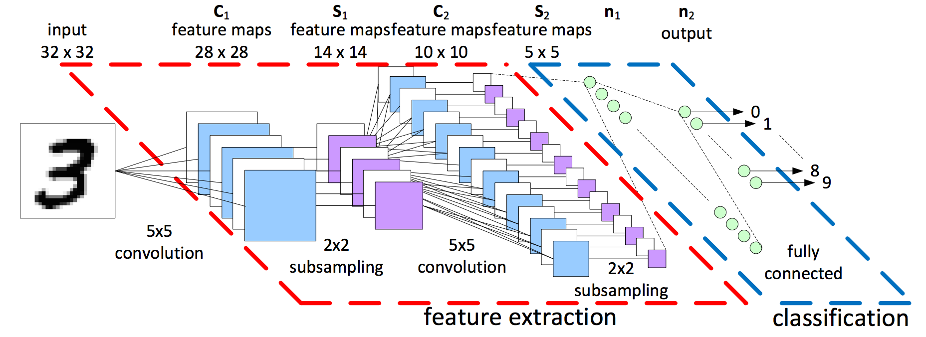
Convolutional Neural Network (CNN) consists of Convolutional Layer, Pooling Layer and Fully Connected Layer. in Convolutional Layer, the kernel(collection of weight) will scan input data with particular stride(moving step) like below picture.
in above picture, input data is MNIST dataset with size 28x28. data will be put into convolutional layer -> max pooling layer and so on. in Fully connected layer, the data will be changed into flat size (one dimension) and enter into next layer until shrink into output layer which is consists of 10 class.
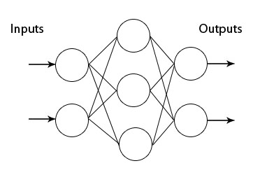
Multilayer Perceptron (MLP) or DNN consists of fully connected layers that connected each other like below picture:
input MNIST data from 28x28 pixel will be changed into flat data (784 pixel). each pixels occupy one neuron in input and forward through network until shrink into 10 class.
- Import Library
import torch #import torch library
import torch.nn as nn #import torch neural network library
import torch.nn.functional as F #import functional neural network module
import torch.optim as optim #import optimizer neural network module
from torch.autograd import Variable #import variable that connect to automatic differentiation
from torchvision import datasets, transforms #import torchvision for datasets and transform- Defining Multilayer Perceptron Model Class
class DNN(nn.Module):
	def __init__(self):
		super(DNN, self).__init__() #load super class for training data
		self.fc1 = nn.Linear(784, 320) #defining fully connected with input 784 and output 320
		self.fc2 = nn.Linear(320, 50) #defining fully connected with input 320 and output 50
		self.fc3 = nn.Linear(50, 10) #defining fully connected with input 50 and output 10
		self.relu = nn.ReLU() #defining Rectified Linear Unit as activation function

	def forward(self, x): #feed forward
		layer1 = x.view(-1, 784) #make it flat in one dimension from 0 - 784
		layer2 = self.relu(self.fc1(layer1)) #layer2 = layer1 -> fc1 -> relu
		layer3 = self.relu(self.fc2(layer2)) #layer3 = layer2 -> fc2 -> relu
		layer4 = self.relu(self.fc3(layer3)) #layer4 = layer3 -> fc2 -> relu
return F.log_softmax(layer4) #softmax activation to layer4- Defining Convolutional Neural Network Model Class
class CNN(nn.Module):
	def __init__(self):
		super(CNN, self).__init__() #load super class for training data
		self.conv1 = nn.Conv2d(1, 10, 5) #Convolutional modul: input 1, output 10, kernel 5
		self.conv2 = nn.Conv2d(10, 20, 5) #Convolutional modul: input 10, output 20, kernel 5
		self.maxpool = nn.MaxPool2d(2) #maxpooling modul: kernel
		self.relu = nn.ReLU() #activation relu modul
		self.dropout2d = nn.Dropout2d() #dropout modul
		self.fc1 = nn.Linear(320, 50) #Fully Connected modul: input, output
		self.fc2 = nn.Linear(50, 10)# Fully Connected modul: input, output

	def forward(self, x): #feed forward
		layer1 = self.relu(self.maxpool(self.conv1(x))) # layer1 = x -> conv1 -> maxpool -> relu
		layer2 = self.relu(self.maxpool(self.dropout2d(self.conv2(layer1)))) #layer2 = layer1 -> conv2 -> dropout -> maxpool -> relu
		layer3 = layer2.view(-1, 320) #make it flat from 0 - 320
		layer4 = self.relu(self.fc1(layer3)) #layer4 = layer3 -> fc1 -> relu
		layer5 = self.fc2(layer4) #layer5 = layer4 -> fc2
return F.log_softmax(layer5) #softmax activation to layer5- Defining Dataset Class
class Dataset:
	def read(self):
		#load train and test loader that the range will be normalized into 0-1, batch size=1000 and shuffle the data
		train_loader = torch.utils.data.DataLoader(
			datasets.MNIST('dataset/',train=True, download=False,
				 transform=transforms.Compose([transforms.ToTensor(),transforms.Normalize((0.1307,), (0.3081,))])),
				 batch_size=1000, shuffle=True)
		test_loader = torch.utils.data.DataLoader(
			datasets.MNIST('dataset/',train=False,
				 transform=transforms.Compose([transforms.ToTensor(),transforms.Normalize((0.1307,), (0.3081,))])),
				 batch_size=1000, shuffle=True)
return train_loader, test_loader- select model
model = CNN() #or you can choose: model = DNN()- read dataset
train_loader,test_loader = Dataset().read() #read dataset from Dataset class that we've defined before and store into train_loader and test_loader- Define Optimizer
optimizer = optim.SGD(model.parameters(), lr=0.01, momentum=0.9) #load optimizer Stochastic Gradient Descent with momentum 0.9 and learning rate 0.01- Loop per epoch and Update Weight
for epoch in range(int(args['epoch'])): # train epoch = 10
		model.train() #training
		for batch_idx, (data, label) in enumerate(train_loader): #enumerate train_loader per batch-> index, (data, label) ex: 0, (img1, 4)... 1, (img2, 2)
			data, label = Variable(data), Variable(label) #create torch variable and enter each data and label into it
			optimizer.zero_grad()
			output = model(data) #enter data into model, save in output
			train_loss = F.nll_loss(output, label) #nll = negative log likehood loss between output and label. it useful for classification problem with n class
			train_loss.backward() #compute gradient
			optimizer.step() #update weight
			if batch_idx % 10 == 0: #display step
				print('Train Epochs: {}, Loss: {:.6f} '.format(epoch, train_loss.data[0] )) #print
		model.eval() #evaluation/testing
		test_loss = 0
		correct = 0
		for data, label in test_loader: #separate data and label
			data, label = Variable(data,volatile=True), Variable(label) #create torch variable and enter data and label into it
			output = model(data) #enter data into model, save in output
			test_loss += F.nll_loss(output, label, size_average=False).data[0] #
			pred = output.data.max(1, keepdim=True)[1] #prediction result
			correct += pred.eq(label.data.view_as(pred)).cpu().sum() #if label=pred then correct++
		test_loss /= len(test_loader.dataset) #compute test loss
print('\nAverage Loss: {:.4f}, Accuracy: {:.0f}'.format(test_loss, 100. * correct / len(test_loader.dataset)))We can see from below picture, loss CNN is better than MLP. After training, i can produce accuracy 96% with CNN and 86 with MLP.


