User guide

In this section a short manual is presented that should allow users to get started with XMI-MSIM. Although the screenshots were obtained on a Mac, they should be representative for Windows and Linux as well. Significant differences will be indicated. The following guide assumes that the user has already installed XMI-MSIM, according to the Installation instructions.

• Launching XMI-MSIM
• Creating an input-file
• Saving an input-file
• Starting a simulation
• Visualizing the results
• Global preferences
• Checking for updates
• Command line interface
• Example files

Launching XMI-MSIM

For macOS users: assuming you dragged the app into the Applications folder, use Finder or Spotlight to launch XMI-MSIM. If you get a dialog complaining about XMI-MSIM being untrusted, you will need to right-click the app icon and click 'Open' where there will be an option to open the app anyway. Afterwards, you will not have to do this again. The warning is due to me not signing the app with an Apple issued certificate, for which I would need to pay $100 US a year...

For Windows users: an entry should have been added to the Start menu. Navigate towards it in Programs and click on XMI-MSIM.

For Linux users: an entry should have been added to the Education section of your Start menu. Since this may very considerably depending on the Linux flavor that is being used, this may not be obvious at first. Alternatively, fire up a terminal and type:

xmimsim-gui

Your desktop should now be embellished with a window resembling the one in the following screenshot.

XMI-MSIM may also be started on most platforms by double clicking XMI-MSIM input-files (.xmsi extension) and output-files (.xmso extension) in your platform's file manager, thereby loading the file's contents.

The main window of the XMI-MSIM GUI consists of three pages that each serve a well-defined purpose. The first page is used to generate inputfiles, based on a number of parameters that are defined by the user. The second page allows for the execution of these files, while the third and last page is designed to visualise the results and help in their interpretation. The purpose of the following sections is to provide an in-depth guide on how to operate these pages.

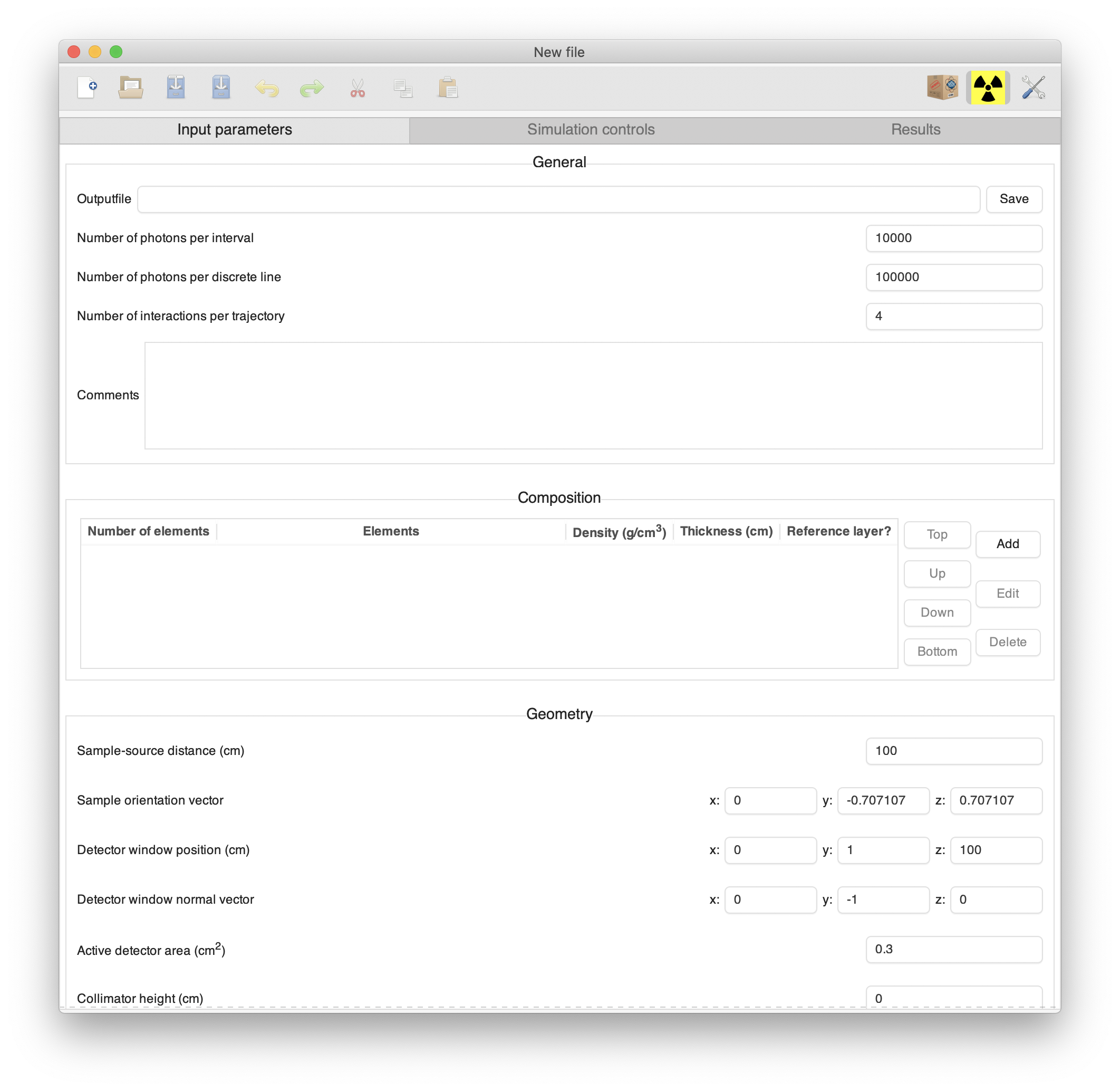
When starting XMI-MSIM without providing a file to open, a new file will be started with default settings. The same situation can be obtained at any moment by clicking on New in the toolbar.

Creating an input-file

The first page consists of a number of frames, each designed to manipulate a particular part of the parameters that govern a simulation.

• General
• Composition
• Geometry
• Excitation
• Beam and detection absorbers
• Detector settings

General

The General section contains 4 parameters:

• Outputfile: clicking the Save button will pop up a file chooser dialog, allowing you to select the name of the outputfile that will contain the results of the simulation
• Number of photons per discrete line: the excitation spectrum as it is used by the simulation may consist of a number of discrete components with each a given energy and intensity (see Excitation for more information). This parameter will determine how many photons are to be simulated per discrete line. The calculation time is directly proportional to this value
• Number of photons per interval: the excitation spectrum as it is used by the simulation may consist of a number of continuous interval components defined by the given energies and intensity densities at the beginning and the end of the intervals (see Excitation for more information). This parameter will determine how many photons are to be simulated per interval. The calculation time is directly proportional to this value
• Number of interactions per trajectory: this parameter will determine the maximum number of interactions a photon can experience during its trajectory. It is not recommended to set this value to higher than 4, since the contribution of increasingly higher order interactions to the spectrum decreases fast. The calculation time is directly proportional to this value
• Comments: use this textbox to write down some notes you think are useful.

Composition

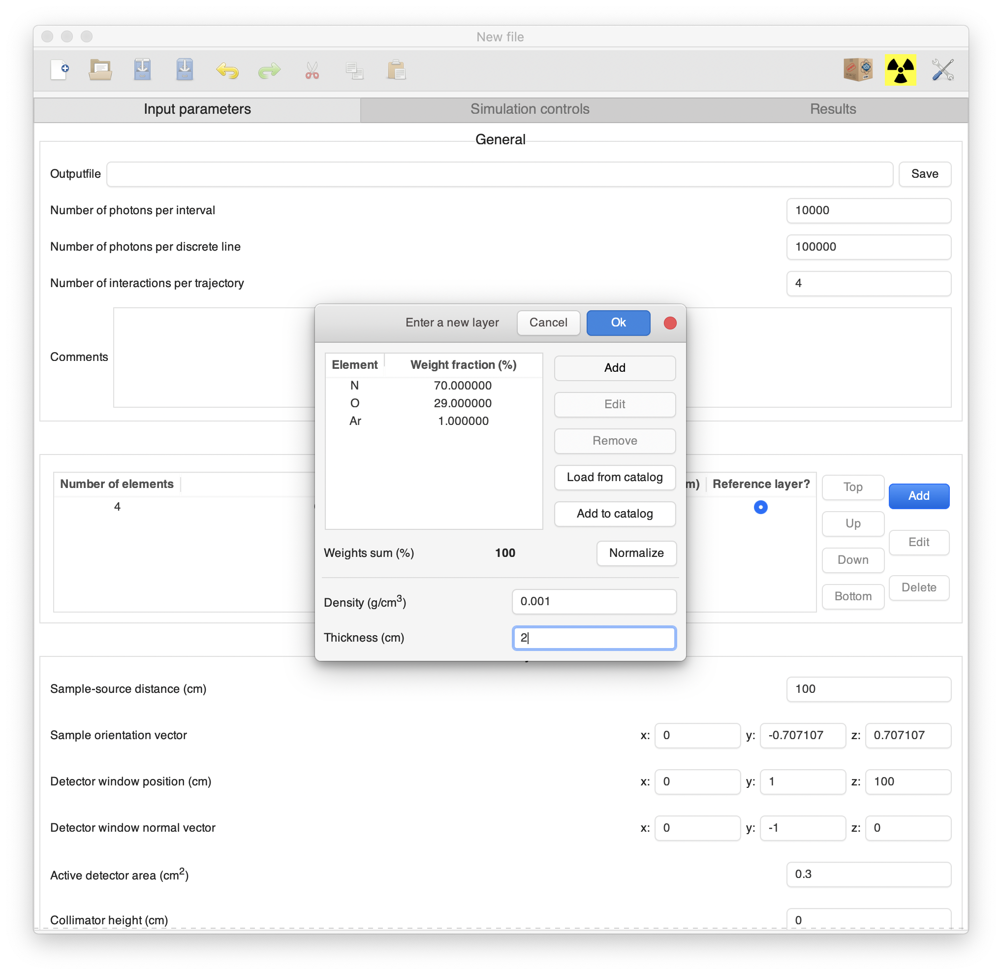
This interface allows you to define the system that will make up your sample and possibly its environment. XMI-MSIM assumes that the system is defined as a stack of parallel layers, each defined by its composition, thickness (measured along the Sample orientation vector) and density. Adding layers can be accomplished by simply clicking the Add button. A dialog will pop up as seen in the following screenshot:

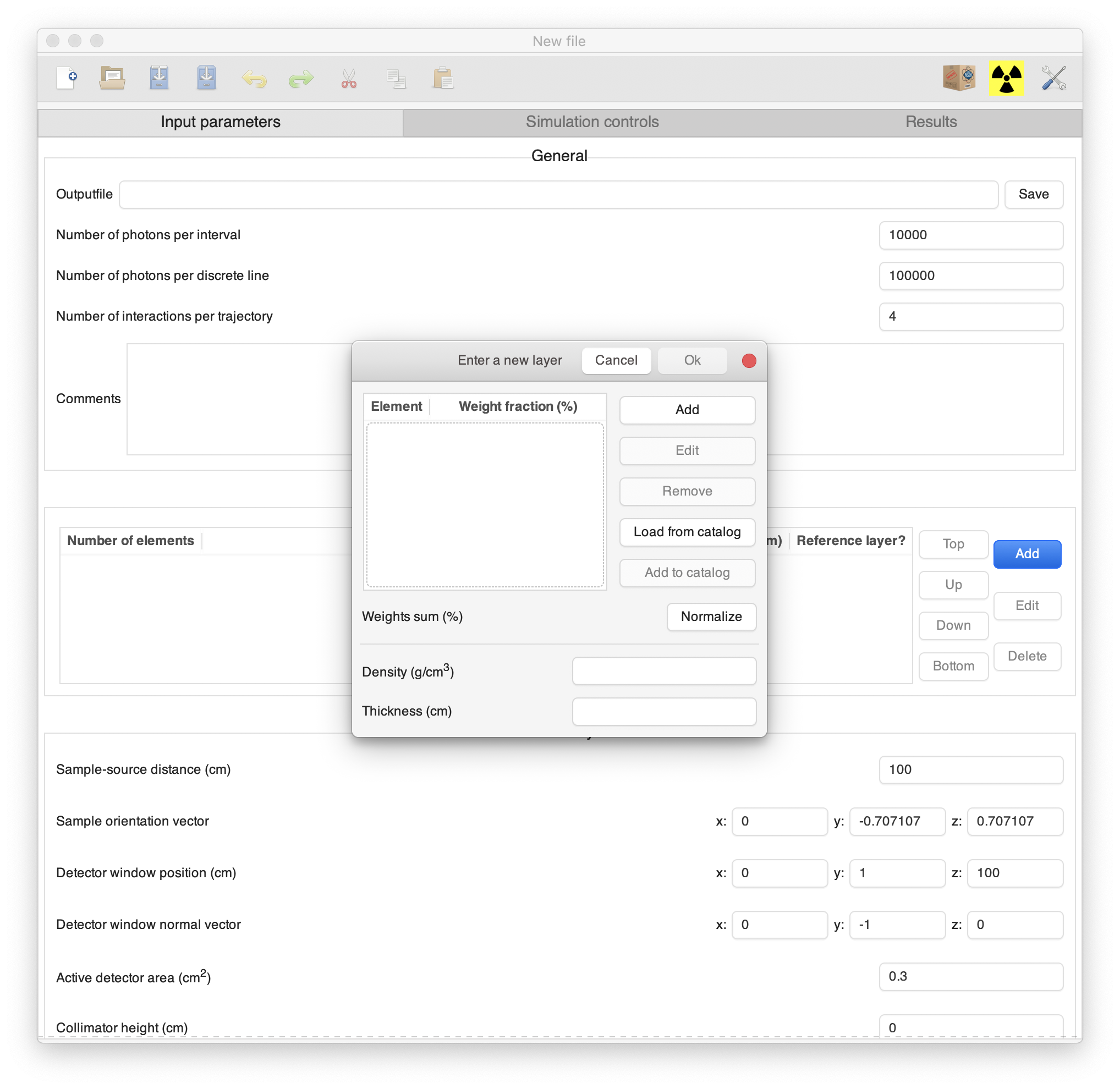
The different elements that make up the layer are added by clicking on the Add button. A small dialog will emerge, enabling you to define a compound or a single element, with its corresponding weight fraction. In the following screenshot, I used CuSO4 with a weight fraction of 50 % to start with.

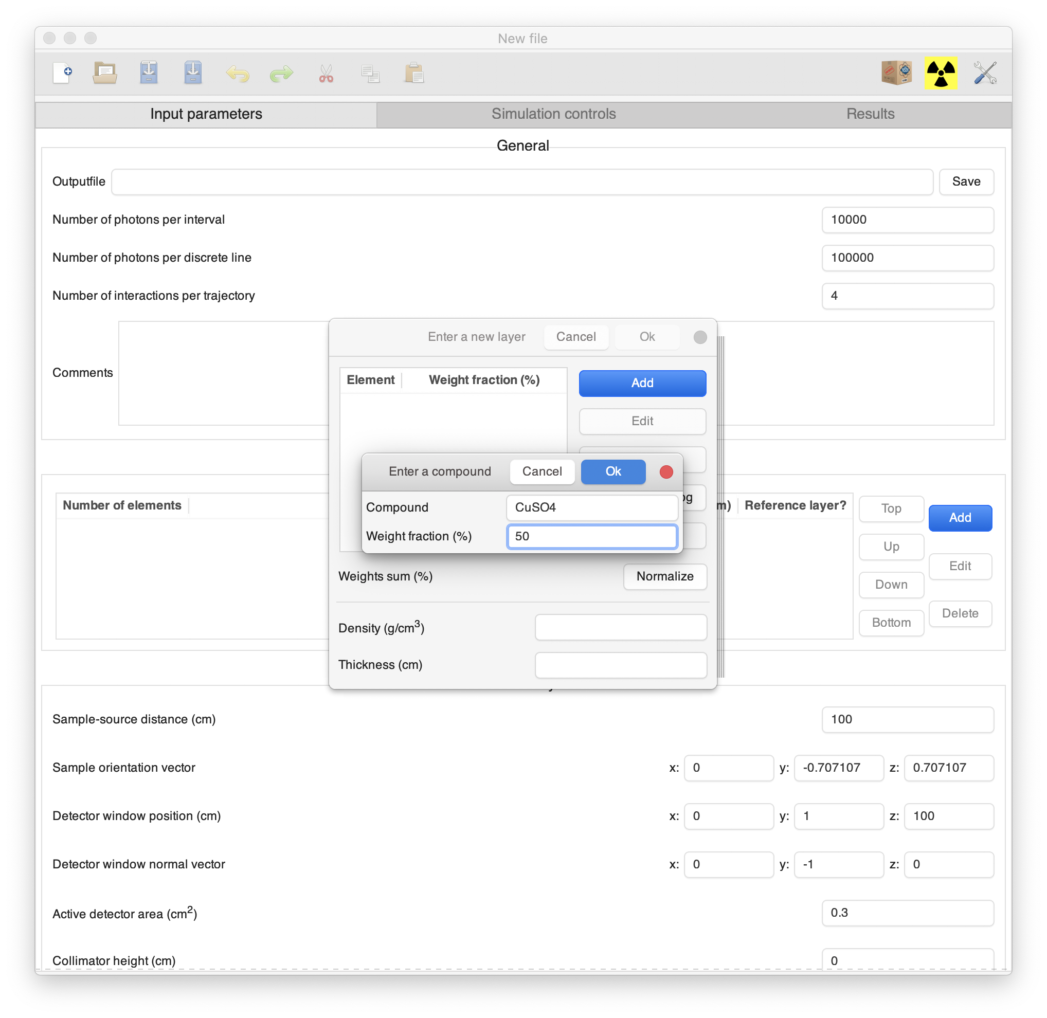
You may wonder at exactly which chemical formulas are accepted by the interface. Well the answer is: anything that is accepted by xraylib's CompoundParser function. This includes formulas with (nested) brackets such as: Ca10(PO4)3OH (apatite). Invalid formulas will lead to the Ok button being greyed out and the Compound text box gaining a red background.

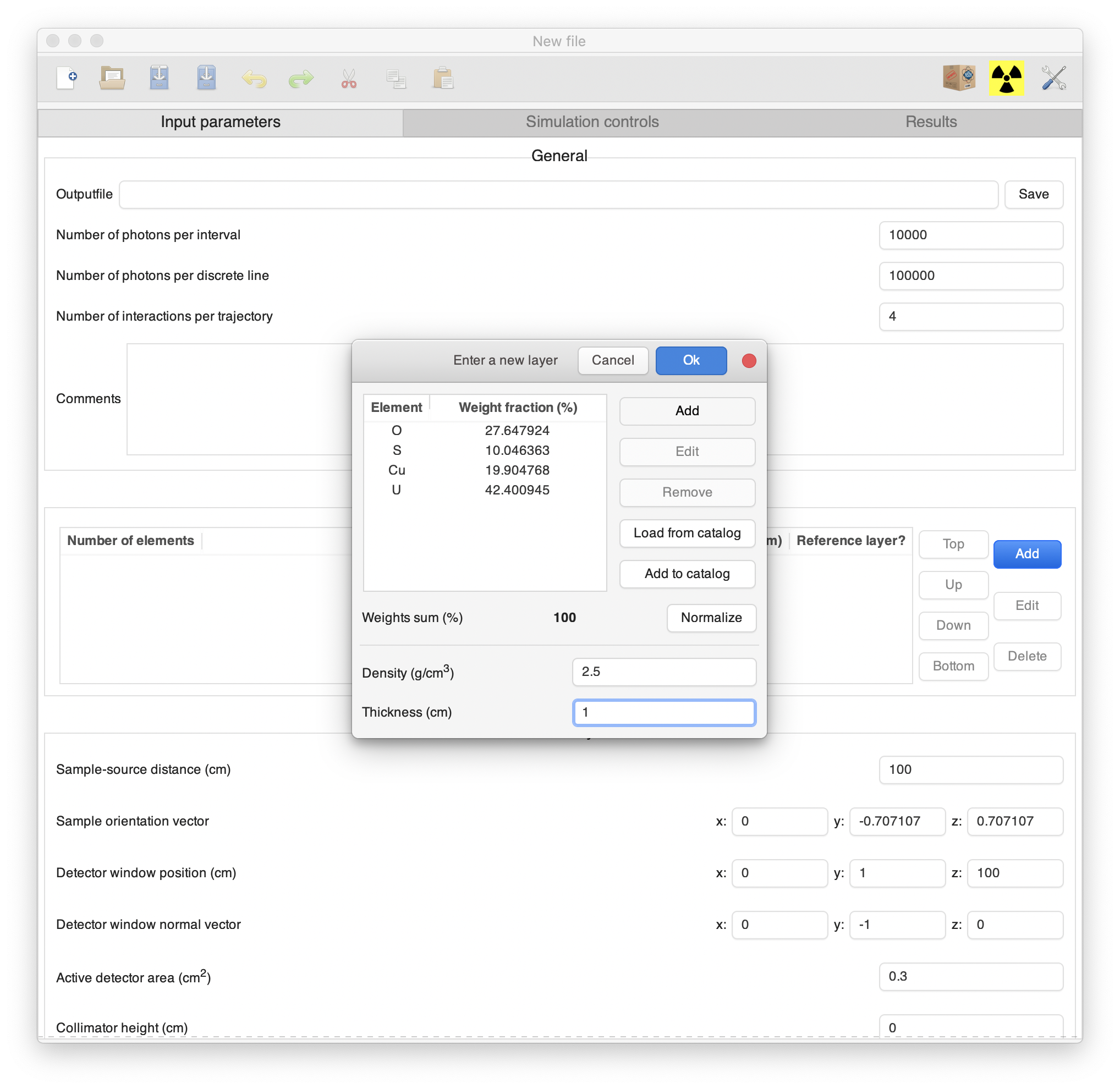
After clicking ok, you should see something resembling the following screenshot:

You will notice that the compound has been parsed and separated into its constituent elements, with weight fractions according to the mass fractions of the elements. In this example I added an additional 50 % of U3O8 to the composition and picked the values 2.5 g/cm3 and 1 cm for density and thickness, respectively, leading to a weights sum of 100 %. It is considered good practice to have the weights sum equal to 100 %. This can be accomplished by either adding/editing/removing compounds and elements from the list, or by clicking the Normalize button, which will scale all weight fractions in order to have their sum equal to 100 %. Your dialog should match with this screenshot:

Alternatively you may consider looking into the builtin catalog (press Load from catalog): a pop-up window will allow you to select a compound from one of two lists. The first list is generated using xraylib's GetCompoundDataNISTList function, which provides access to NISTs compound database of compositions and densities. The second one however, provides access to layers that you defined yourself: when a valid layer (i.e. composition, density and thickness) is showing in the layer dialog, click Add to catalog and choose a name for the layer: this layer will show up in the catalog list next time it is opened. Keep in mind that existing layers in the list will be overwritten without warning! If you would like to delete previously defined layers from the list, use the Preferences interface.

When satisfied with the layer characteristics, press Ok.

X-ray fluorescence experiments are quite often performed under atmospheric conditions. If so, it is of crucial importance to add the atmosphere to the system for several reasons:

1. The atmosphere attenuates the beam and the X-ray fluorescence
2. The intensity of the Rayleigh and Compton scatter peaks is greatly influenced by the atmosphere
3. The photons from the beam as well as the fluorescence and the scattered photons will lead to the production of Ar-K fluorescence, a common artefact in X-ray fluorescence spectra. In some rare cases, one may even detect Xe fluorescence.

To add such a layer, click again on Add button. In the Modify layer dialog, add the composition, density and thickness of the air layer. This is shown in the next screenshot:

Alternatively, click on Load from catalog and select Air, Dry (near sea level) from the NIST compositions list. Clicking the Ok button should produce the following situation in the Composition section:

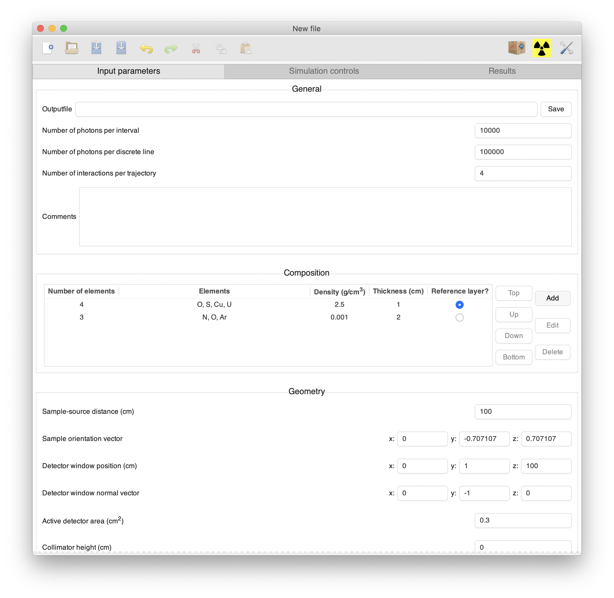
However, the ordering of the layers in the table is wrong: XMI-MSIM assumes that the layers are ordered according to distance from the X-ray source. This means that the first layer is closest to the source and all subsequent layers are positioned at increasingly greater distances from the source. This can be easily remedied by selecting a layer and then moving it around using the Top, Up, Down and Bottom buttons. The following screenshot shows the corrected order of the layers:

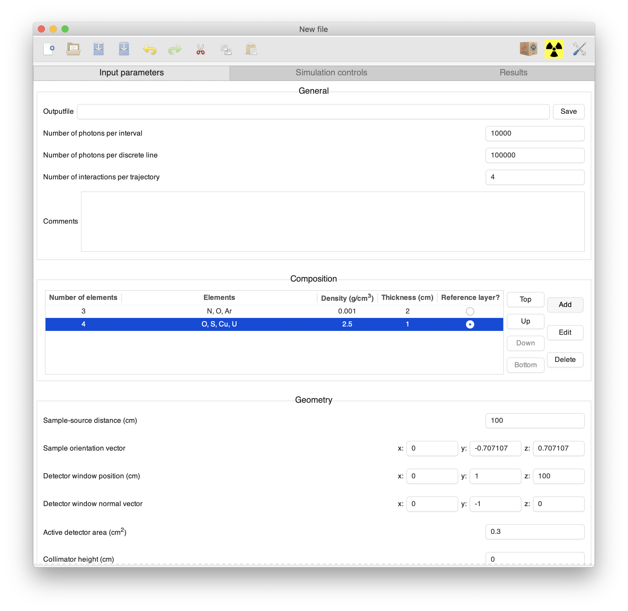
An important parameter in this table is the Reference layer. Using the toggle button, you select which layer corresponds to the one that is considered to be the first layer of the actual sample. In most cases, this will indicate the first non-atmospheric layer. The Reference layer is also the layer that is used to calculate the Sample-source distance in the Geometry section.

Layers can be removed by selecting them and then clicking the Remove button. Existing layers may be modified by either double-clicking the layer of interest or by selecting the layer, followed by clicking the Edit button.

Keep in mind that the number of elements influences the computational time greatly, especially when dealing with high Z-elements that may produce L- and M-lines.

Geometry

Scrolling down a little on the Input parameters page reveals the Geometry section as shown in the next screenshot:

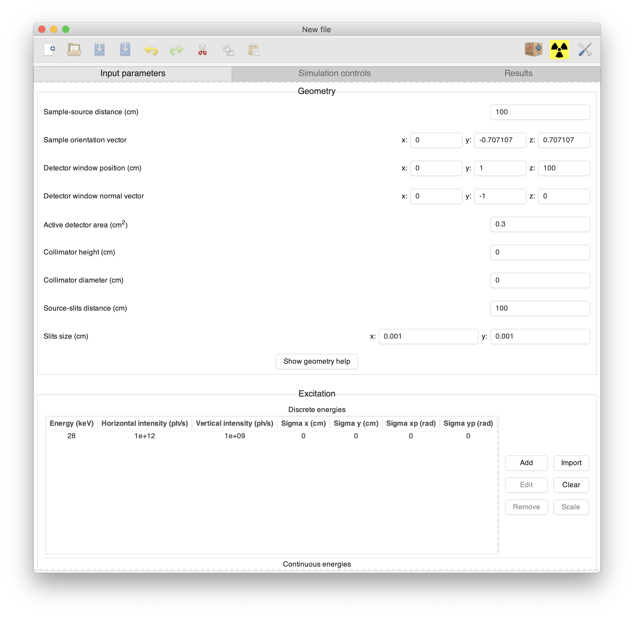
This sections covers the position and orientation of the system of layers, detector and slits. In order to fully appreciate the geometry parameters, it is important that I first describe the coordinate system that these position coordinates and directions are connected to:

• The coordinate system is right-handed Cartesian
• The origin of the coordinate system corresponds to the position of the source
• The z-axis is aligned with the beam direction and points from the source towards the sample
• The y-axis defines, along with the z-axis, the horizontal plane
• The x-axis emerges out from the plane formed by the y- and z-axes

This is demonstrated in the following figure:

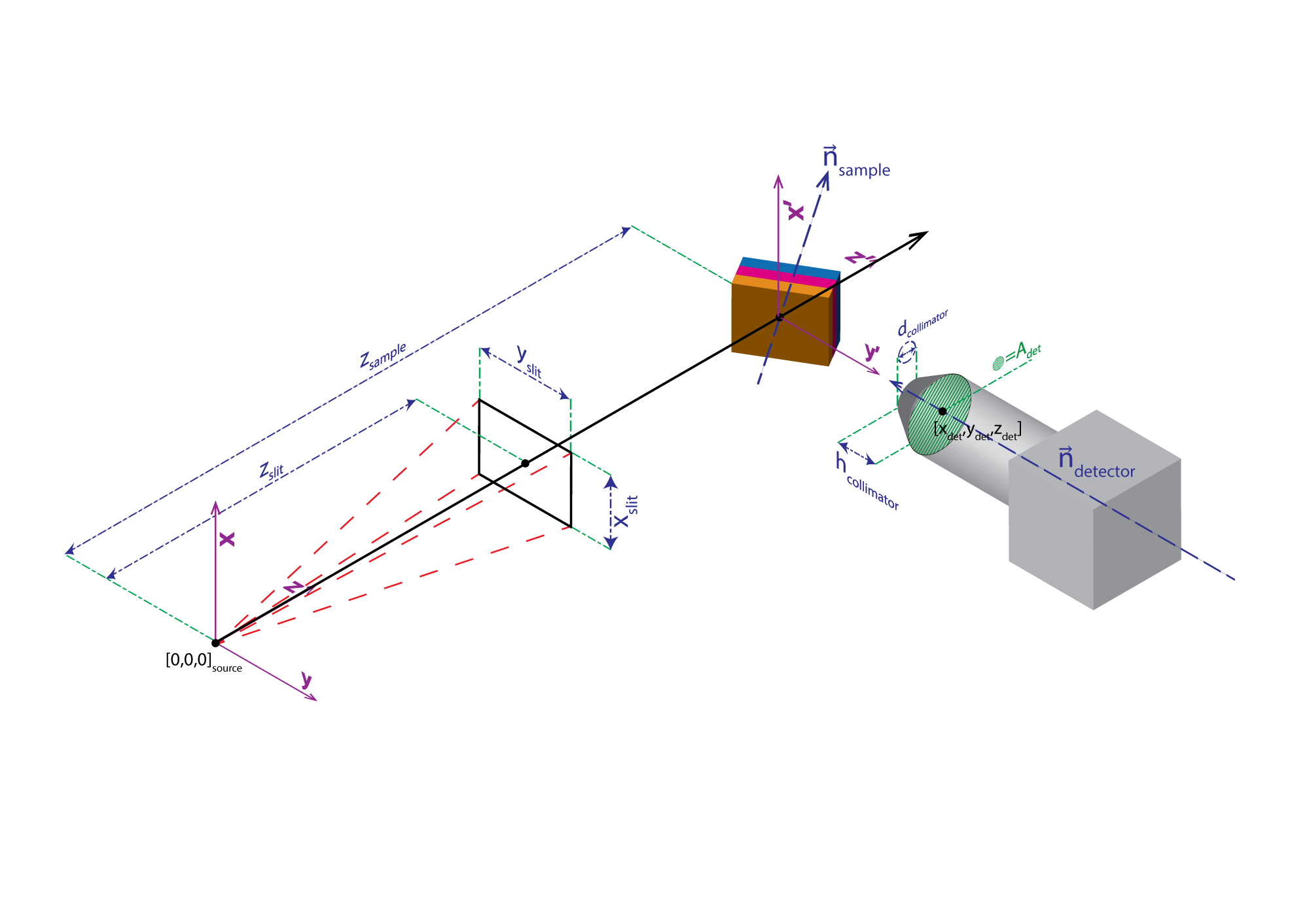
Now with this covered, let us have a look at the different Geometry parameters:

• Sample-source distance: the distance between the source and the Reference layer in the system of layers as defined in the Composition section
• Sample orientation vector: the normal vector that determines the orientation of the stack of layers that define the sample and its environment. The z component must be strictly positive
• Detector window position: the position of the detector window. This is seen as the point where the photons are actually detected and terminated by the detector. Keep this in mind when defining a collimator
• Detector window normal vector: the normal vector of the detector window. Should be directed towards the sample (unless you have a very good reason not to do so)
• Active detector area: this corresponds to the area of the detector window that is capable of letting through detectable photons. Should be provided by the manufacturer of your detector
• Collimator height: XMI-MSIM allows for the definition of a conical detector-collimator whose properties are determined by this parameter and the Collimator diameter. Setting either to zero corresponds to a situation without collimator. This height parameter is seen as the height of the cone, measured from the detector window to the opening of the collimator, along the detector window normal vector
• Collimator diameter: diameter of the opening of the conical detector collimator. The base of the collimator corresponds to the Active detector area
• Source-slits distance: XMI-MSIM defines a set of virtual slits, whose purpose is to define the size of the beam at a given point, based on the distance between these slits and the X-ray source, as well as the Slits size, defined by the next parameter. I recommend to have the Source-slits distance correspond to the Sample-source distance, since this way the beam, upon hitting the Reference layer, will have exactly the dimensions specified by Slits size (if using a point source!). These slits should not be thought of as physical slits, as they are often encountered in many experimental setups: XMI-MSIM's virtual slits do not reduce the beam intensity (flux) at all! They do impact the flux density which increases when decreasing the Slits size parameters, and vice versa.
• Slits size: see previous parameter. Refers to the dimensions of the beam at the Source-slits distance. This parameter will be ignored when dealing with a Gaussian source (see Excitation section)

In order to visualize these different parameters, click the Show geometry help button: a new window will pop up showing the aforementioned coordinate system. Hovering the mouse over the different components in the new window will have the corresponding widgets light up in green in the main window. This works both ways: hover the mouse over the geometry widgets in the main window and little boxes will appear in the coordinate system window.

Excitation

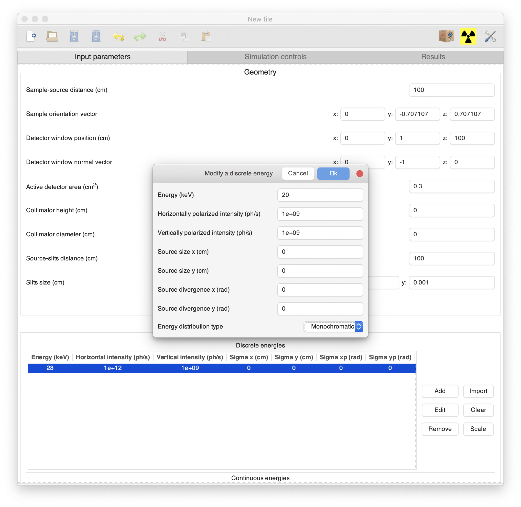
Next, there is the Excitation section, which is used to define the X-ray beam that irradiates the sample. The corresponding excitation spectrum may consist of a number of discrete components, each with a horizontally and vertically polarized intensity, as well as a number of parameters that define the type and the aperture of the source. Furthermore, one can also insert a number of continuous interval components, defined through a list of intensity densities, each with their horizontally and vertically polarized components. In this case, one has two insert at least two intensity densities in order to have at least one interval.

At runtime, the code will use the Number of photons per discrete line and Number of photons per interval parameters to determine how many photons will be simulated per discrete component and continuous energy interval component. Adding, editing and removing components is handled through the buttons in the Excitation section. For example, we can change the settings of the default value by clicking the Edit button. The dialog contains the fields necessary to define a particular component:

• Energy: the energy of this particular part of the excitation spectrum, expressed in keV
• Horizontally and vertically polarized intensities: the number of photons that are polarized in the horizontal and vertical planes, respectively. A completely unpolarized beam has identical horizontal and vertical intensities (such as those produced by X-ray tubes), while synchrotron beams will have very, very low vertically polarized intensities. For information on how to convert the total number of photons given the degree of polarization to the horizontal and vertical polarized intenties, consult Part 5 in our series of papers on Monte-Carlo simulations
• Source size x and y: if both these values are equal to zero, then the source is assumed to be a point source, and the divergence of the beam is completely determined by the Source-slits distance and Slits size parameters of the Geometry section. Otherwise the source is considered a Gaussian source, in which case the photon starting position is chosen according to Gaussian distributions in the x and y planes, determined by the Source size x and Source size y parameters
• Source divergence x and y: if these values are non-zero, AND the source is Gaussian, then the Source-slits distance takes on a new role as it becomes the distance between the actual focus and the source position. In this way a convergent beam can be defined, emitted by a Gaussian source at the origin. For the specific case of focusing on the sample the Sample-source distance should be set to the Source-slits distance.
• Energy distribution type: additionally for the discrete components, it is possible to set the Energy distribution type, which may assume the values Monochromatic, Gaussian and Lorentzian. The first case assumes that the discrete energy is purely monochromatic and that only the selected energy will be used in the simulation. The two other cases corrspond to a scenario in which the simulation will sample from a Gaussian or Lorentzian distribution respectively. If either of these two cases is selected, the user is expected to provide respectively the standard deviation and the scale parameter.

In this particular case, I have changed the energy to 20.0 keV, and made the beam unpolarized by equalizing both intensities, as shown in the following screen shot. The source remains a point source.

The discrete energies and continuous energies widgets each contain six buttons:

• Add: add a new component.
• Edit: edit a previously defined component.
• Remove: delete previously components.
• Import: import a list of discrete lines or continuous energy intensity densities from an ASCII file. These files must consist of either two, three or seven columns, with the first column containing the energies, the second the total intensity (if only two columns are found), or the second and third the resp. horizontally and vertically polarized intensities or intensity densities. If seven columns are encountered, the last four columns are assumed to contain source sizes and divergencies. It is possible through the interface to start reading only at a certain linenumber and also to read only a set number of lines.
• Clear: delete all previously defined components.
• Scale: multiply the intensities or intensity densities with a positive real number.

The excitation spectrum can also be defined using the X-ray sources dialog.

Beam and detection absorbers

The two following sections deal with absorbers, first absorbers that are optionally placed in the excitation path (for example a sheet of Al or Cu), and next the absorbers that are optionally placed in the detector path. This means that the former will reduce the intensity of the incoming beam, while the latter will reduce the intensity of the photons that hits the detector. It is important to realize that these absorbers are only used here for their attenuating properties, they are not considered as objects in the simulations so they cannot contribute fluorescence lines to the eventual spectrum! Adding, editing and removing absorbers is performed through an interface identical to the one seen in the Composition section, but without the Reference layer toggle button. New inputfiles will always have a Be detector absorber added, corresponding to the detector window commonly found in ED-XRF detectors.

Detector settings

The last section deals with the settings of the detector and its associated electronics, as can be seein in the following screenshot:

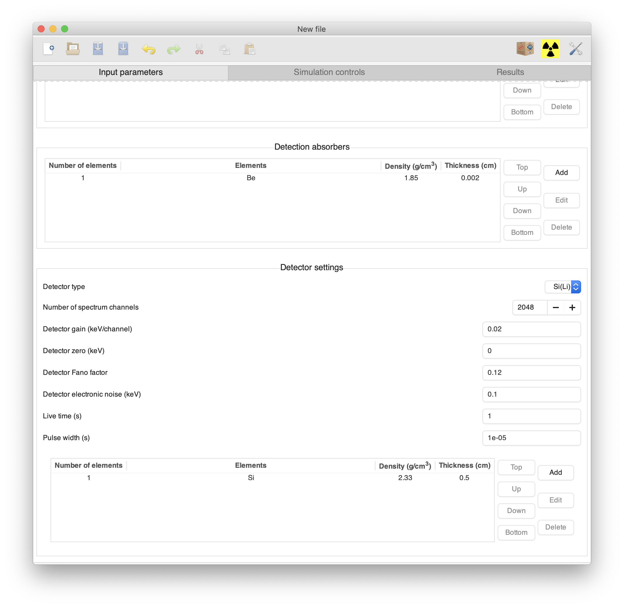
• Detector type: every detector comes with its own detector response function, which can be influenced by several detector and electronics parameters. XMI-MSIM offers some predefined detector response functions that its authors have found to be reasonably well for two detector types: Si(Li) and Si Drift Detectors. Generally speaking, our policy is to encourage users to implement their own detector response functions in the form as a plug-in and load it in the Simulation options
• Number of spectrum channels: the number of channels in the produced spectrum
• Live time: the actual measurement time of the simulated experiment, taking into account dead time
• Detector gain: the width of one channel of the spectrum, expressed in keV/channel
• Detector zero: the energy of the first channel in the spectrum (channel number zero)
• Detector Fano factor: measure of the dispersion of a probability distribution of the fluctuation of an electric charge in the detector. Very much detector type dependent
• Detector electronic noise: the result of random fluctuations in thermally generated leakage currents within the detector itself and in the early stages of the amplifier components. Contributes to the Gaussian broadening
• Pulse width: the time that is necessary for the electronics to process one incoming photon. This value will be used only if the user enables the pulse pile-up simulation in the Simulation controls. Although this parameter is connected to several detector and electronics parameters, typically the value is obtained after trial and error
• Crystal composition: the composition of the detector crystal. Adding, editing and removing absorbers is performed through an interface identical to the one seen in the Composition section, but without the Reference layer toggle button. Will be used to calculate the detector transmission and the escape peak ratios

Saving an input-file

Once an acceptable inputfile is detected by the application, the Save and Save As buttons will become activated. If the file has not been saved before, clicking either of these buttons will launch a dialog allowing you to choose a filename for the input-file.

If the file was saved before, then clicking Save will result in the file contents will be overwritten with the new file contents.

Keep in mind that XMI-MSIM input-files have the xmsi extension (blue logo), while the output-files the xmso extension (red logo).

Starting a simulation

• Control panel
• Executable
• Options
• Export results
• During a simulation

In order to start a simulation, the Input parameters page must contain a valid input-file description. This can be obtained by either preparing a new input-file based on the instructions in a previous section (and saving it!), or by opening an existing input-file by double clicking an XMI-MSIM input-file in your file manager or opening an input-file through the Open interface of XMI-MSIM.

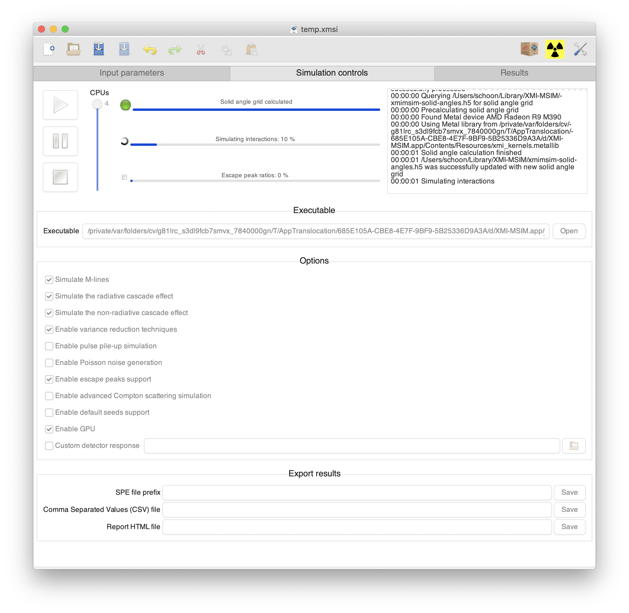
Either way, the Simulation controls page should look as shown in the following screenshot:

Control panel

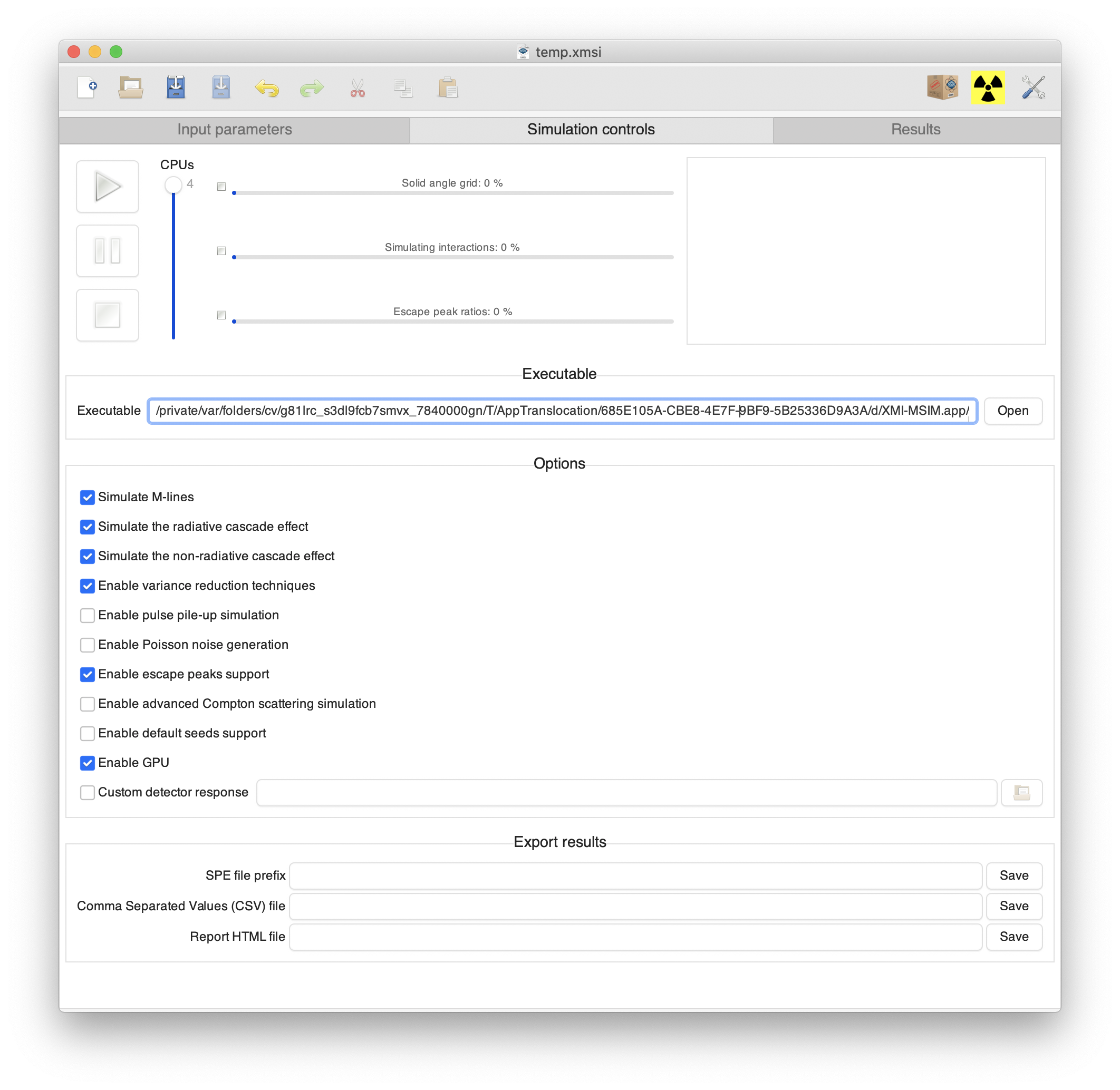
The top of the page contains the actual control panel that is used to start, stop and pause the simulation, as well as a slider that allows the user to select the number of threads that will be used by the simulation. To the right of the slider, there are three progress bars that indicate different stages of the Monte Carlo program: the calculation of the solid angle grid for the variance reduction, the simulation of the photon--matter interactions and the calculation of the escape peak ratios. More information about the status of the Monte Carlo program is presented in the adjacent log window.

Executable

Underneath these controls is a section that contains the name of the executable that will be used to launch the simulation. Most likely, you will never have to change this value, but it could be interesting to power users, who have customized versions of the simulation program.

Options

This section is followed by a number of options that change the behaviour of the Monte Carlo program:

• Simulate M-lines: If disabled, then the code will ignore M-lines that may be produced based on the elemental composition of the sample. In such a case, the code will probably run faster. I strongly recommend to simulate M-lines
• Simulate the radiative and non-radiative cascade effect: the cascade effect is composed of two components, a radiative and a non-radiative one. Although these will always occur simultaneously in reality, the code allows to deactivate one or both of them. This could be interesting to those that want to investigate the contribution of both components. Otherwise, it is recommended to keep both enabled
• Enable variance reduction techniques: disabling this option will trigger the brute-force mode, disabling all variance reduction techniques, thereby greatly reducing the precision of the estimated spectrum and net-line intensities for a given Number of photons per discrete line. This reduced precision may be improved upon by greatly increasing the Number of photons per discrete line, but this will result in a much longer runtime of the Monte-Carlo program. Expert use only. Consider building XMI-MSIM with MPI support and running it on a cluster
• Enable pulse pile-up simulation: this option activates the simulation of the so-called sum peaks in a spectrum due to the pulse pile-up effect which occurs when more photons are entering the detector than it can process. The magnitude of this effect can controlled through the Pulse width parameter
• Enable Poisson noise generation: enabling this option will result in every channel of the detector convoluted spectrum being subjected to Poisson noise, controlled by Poisson distributions with lambda equal to the number of counts in a channel
• Enable escape peaks support: enable this option to activate the support for escape peaks in the detector response function. Typically you will want to leave this on
• Enable advanced Compton scattering simulation: this option activates an alternative algorithm for the simulation of the Compton profiles based on the work of Fernandez and Scot, which takes into account the fact that not all orbitals are completely populated, leading to a more accurate reproduction of the profiles. The downside of this approach is that it's slower than the default implementation. Recommended only for advanced users. In order to fully understand the importance of an improved Compton profile simulation, the reader is advised to read the aforementioned manuscript of Fernandez and Scot
• Enable default seeds support: instead of using randomly chosen seeds for the random number generators, use default values, which should result in reproducible results, at least when using a single thread. This option should normally not be used.
• Enable GPU: this option invokes XMI-MSIMs GPU plug-in which, if the platform comes with a videocard chipset that supports it, will use the GPU to perform the solid angle calculation, which could lead to a tremendous speed increase. Keep in mind that when this option is used during the solid angle calculation stage, the screen may have a noticeably lower refresh rate and may lose its responsiveness briefly. This option is only available when an OpenCL (all platforms) or Metal (macOS only) framework was found at compile-time
• Custom detector response: through this option, one can load a plug-in that exports a routine that will override the default detector response functions of XMI-MSIM. Click here more information on how to write and build such plug-ins

Export results

The page ends with a section that allows the user to export the output of the Monte-Carlo program at run-time to several fileformats in addition to the default XMSO fileformat.

• SPE file: the well known ASCII format, readable by PyMca and AXIL. Produces one file per additional interaction. When using the file dialog to choose the filename, make sure not to add a file extension: the Monte-Carlo program will append an underscore, the number of interactions and the .spe extension automatically
• Comma Separated Values (CSV) file: produces a CSV file containing several columns. The first column contains the channel number, the second one contains the corresponding channel energy and the following columns contain the intensities for increasing number of interactions
• Report HTML file: produces an html file that can be opened with most Internet Browsers (Internet Explorer being a notable exception), featuring an interactive overview of the results of the Monte-Carlo simulation, simular to the ones shown on the Results page

It is possible to generate these files afterwards based on the XMSO file, by clicking in the menubar on Tools -> Convert XMSO file to.

During a simulation

When all required options are set up correctly, the simulation can be started by clicking the Play button. After this, you will notice a lot of output being generated in the log window, as well as some activity in the progress bars, as shown in the next screenshot:

The first and the third progress bars will in many cases display a message that the Solid angle grid and the Escape peak ratios were loaded from file: this indicates that a simulation with similar parameters was performed before and that the relevant data was written to a file, leading to a huge increase in speed. It is possible that some red text appears during a run, particularly with reference to Solid angle and Escape ratio HDF5 files being outdated. This only happens when you are running a new version of XMI-MSIM that introduced a new format for these files: the old files are deleted and new ones will be created and used from then onwards.

After the simulation, assuming everything went fine, the XMSO outputfile as defined in the General section will be loaded and its contents displayed on the Results page.

Visualizing the results

The results of a simulation are stored in an XMSO file (red logo): you should be able to open these files directly by double clicking them from your file manager. Alternatively, you can also load these files from within XMI-MSIM by clicking the Open button, and subsequently setting the filetype filter to XMI-MSIM outputfiles. On Linux and Windows, you can also open these files from the command-line:

xmimsim-gui file.xmso

XMSO files created after a successful simulation are automatically loaded in the Results page, where the spectra and net-line intensities are represented.

• Plot canvas
• Net-line intensities
• Printing and exporting the plot canvas

Plot canvas

If a simulation was performed according to the inputfile that was defined earlier, you should get a result similar to the one in the following screenshot:

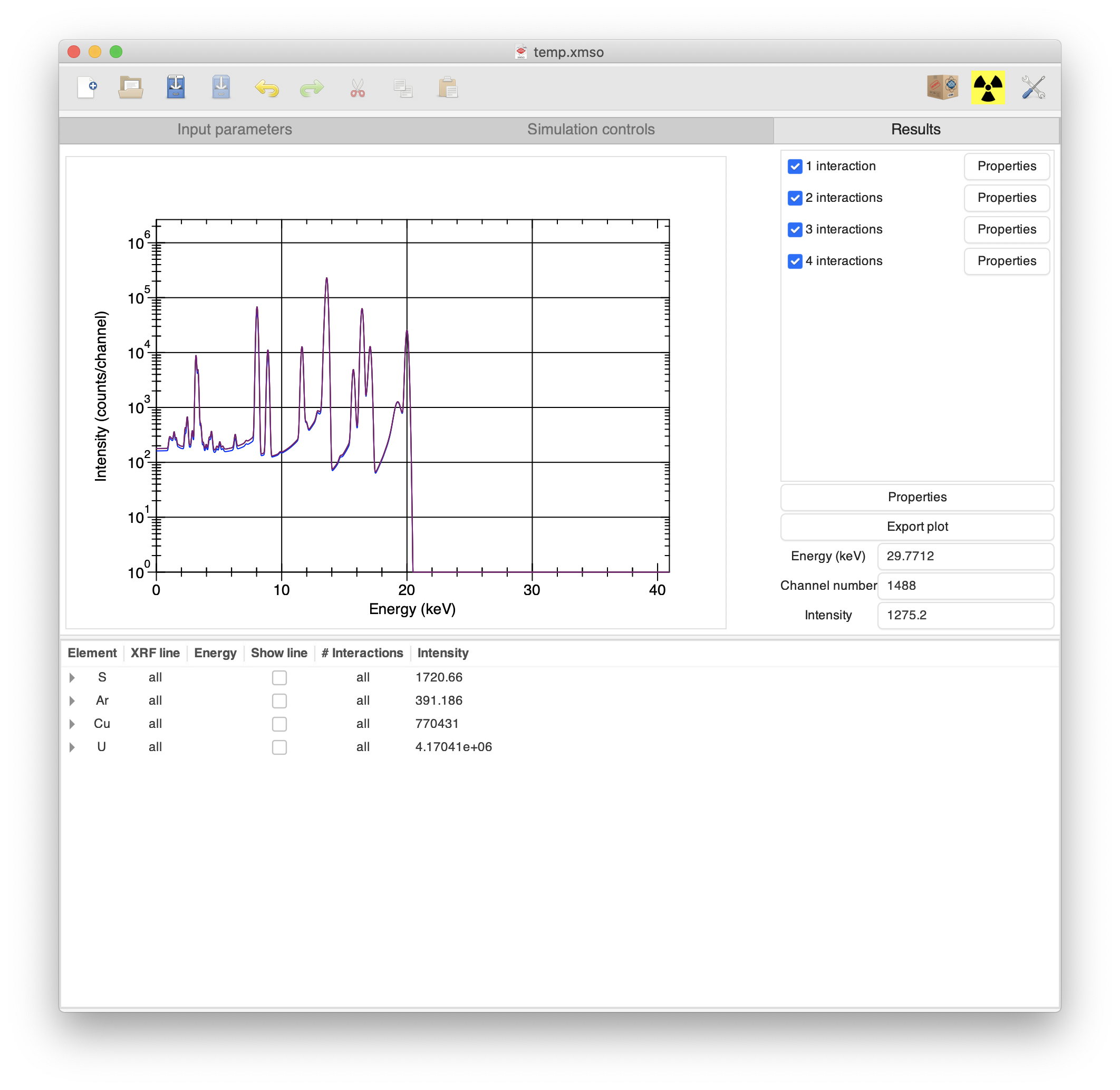
The plot canvas shows by default the different spectra obtained after an increasing number of interactions. Individual spectra may be hidden and shown by toggling the boxes to the right of the plotting window. Their properties of a spectrum may be modified by clicking on the Properties button connected to it, which launches a dialog allowing the user to change the line width, line type and line color of the spectrum. The Properties button above the coordinate entries opens a dialog with the option to switch between linear and logarithmic display of the spectra, as well as the opportunity to change the axes titles. More options will be added in future releases allowing the user to customize this further.

Zooming in on the plot canvas by dragging a rectangle with the mouse while keeping the left button clicked in. Zooming out can be accomplished by double-clicking anywhere in the canvas. While moving the mouse cursor in the plot canvas, one can track the current Energy, Channel number and Intensity in the textboxes to the right. The size of the canvas can be changed by grabbing and moving the handle that separates the upper part from the lower part of the page.

Net-line intensities

The lower part of the page contains a list of all the intensities of all the X-ray fluorescence lines of all elements, as shown in the following screenshot:

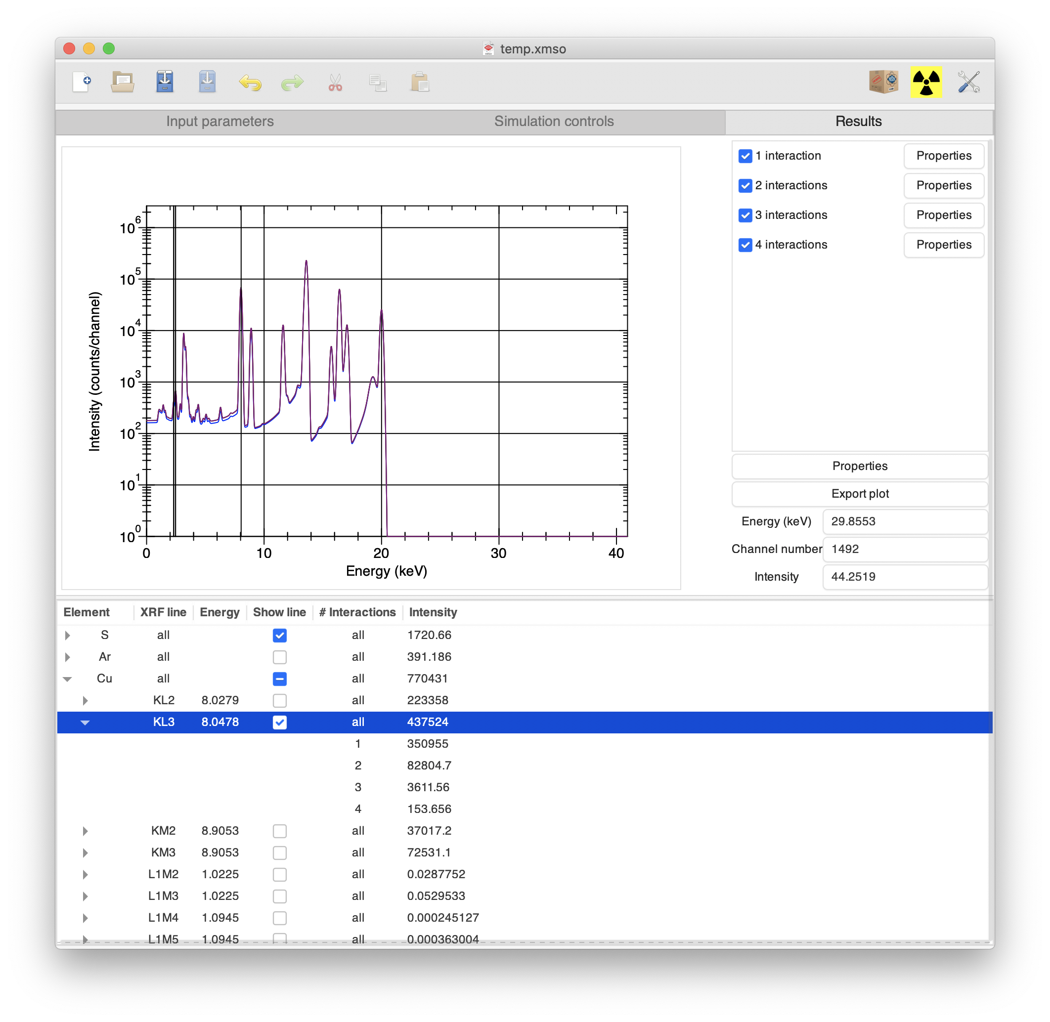
By clicking the arrows on the left side of the list, it is possible to expand the sections belonging to a particular element, line, and for different number of interactions, thereby revealing the individual contributions to a particular intensity. The lines can be shown on the plot canvas by activating the Show line flag for the appropriate line or element.

Exporting the plot canvas

The plot canvas can be exported to several filetypes using the Export plot button to the right of the plot canvas. This will result in an exact copy of the current state of the canvas being stored to file: it will take into account all the changes that were made to the spectra properties, as well as any lines that were activated using the Show line togglebuttons of the Net-line intensities section. Supported filetypes are PNG, EPS, PDF and SVG.

Global preferences

Clicking the Preferences button in the toolbar will launch a dialog allowing the user to set some preferences that will be preserved across sessions off XMI-MSIM. Make sure to press apply after making any changes.

• Simulation defaults
• Updates
• User-defined layers
• Advanced

Simulation defaults

The first page of the preferences window contains the same settings that are available on the Simulation controls page. The values that are selected here will be activated in the Simulation controls page the next time that XMI-MSIM is started.

Updates

If XMI-MSIM was compiled with support for automatic updates then this page will contain two widgets: firstly a checkbox that will determine if the program will check for updates at startup, and secondly a list of locations that will be used to download updates from.

User-defined layers

Select layers and hit backspace to remove them from the list of user-defined layers (which are defined in the layer dialogs). The layers are deleted when the Apply button is clicked.

Advanced

The first two options revolve around the deleting of the XMI-MSIM HDF5 files that contain the solid angle grids and the escape peak ratios, respectively. It is recommended to remove these files manually when a complete uninstall of XMI-MSIM is considered necessary (before running the uninstaller or removing the application manually), or if these files somehow got corrupted.

The following two options allow the user to import solid angle grids and escape peak ratios from external files into his own. This may be interesting if another user already has a huge collection of these and it may save a lot of time using someone elses. In the file dialog only those files will be shown that are valid HDF5 files of the required kind and minimum version.

The last option is Enable notifications, which when supported at compile-time and a suitable notifications server is found, will generate messages whenever a calculation finishes. On a Mac OS X native version of XMI-MSIM this will only work on Mountain Lion and newer.

Checking for updates

For packages of XMI-MSIM that were compiled with support for automatic updates, checking for new versions will occur by default when launching the program. This can be disabled in the Preferences window. If you would like to check explicity, then click on Check for Updates in the toolbar menu. When updates are available, a dialog will pop up, inviting the user to download the package through the interface. When the download is completed, quit XMI-MSIM and install the new version. It is highly recommended to always use the latest version of XMI-MSIM.

Command line interface

XMI-MSIM ships with a number of command line utilities that may be useful for some users. An overview:

• xmimsim-gui: This executable corresponds to the graphical user interface of XMI-MSIM, as described in this user guide. This will mostly be useful for Linux users or Mac OS X users that compiled from source without gtk-mac-integration support.
• xmimsim: The executable that actually does the hard simulation work. It is usually launched from within the graphical user interface with the Play, Pause and Stop buttons from the control panel, but in some circumstances it may be useful from the command-line as well. It has a lot of options: consult them by running xmimsim --help. Windows users will have to use xmimsim-cli.exe since xmimsim.exe is compiled as a graphical user interface executable in order to avoid a console window from popping up during the simulation in XMI-MSIM.
• xmimsim-db: Used to generate the xmimsimdata.h5 file that contains the tables of physical data (mostly inverse cumulative distribution functions) that will be used during the simulation to speed things up drastically. This executable is intended for those that compile XMI-MSIM from source.
• xmimsim-conv: A recently added executable that allows to extract the unconvoluted spectra from an XMSO file and apply the detector response function to it with different settings that were used initially to generate the XMSO file.
• xmimsim-harvester: a daemon that collects seeds for the random number generators. Read the note on the random number generators in the installation instructions for more information.
• xmso2xmsi, xmso2spe, xmso2csv, xmso2htm: utilities that allow for the conversion of XMSO files to the corresponding XMSI, SPE, CSV and HTML counterparts, providing the same functionality as obtained through Tools -> Convert -> XMSO file -> ...
• xmsa2xmso: utility that allows for the extraction of XMSO files from an XMSA file, providing the same functionality as obtained through Tools -> Convert -> XMSA file -> to XMSO.
• xmsi2xrmc: Utility to convert an XMSI file to the corresponding XRMC input-files. Read here for more information. Also available through Tools -> Convert -> XMSI file -> to XRMC input-files.
• xmimsim-pymca: The quantification plug-in that is used by PyMca.

Most of these executables have quite a few options. Consult them by passing the --help option to the executable.

Example files

The example input-file that was created throughout the Creating an input-file section can be downloaded at test.xmsi. The corresponding output-file can be found at test.xmso.