5. Segmentation
Segmentation is a very important processing stage for most of audio analysis applications. The goal is to split an uninterrupted audio signal into homogeneous segments. Segmentation can either be
- supervised: in that case some type of supervised knowledge is used to classify and segment the input signals. This is either achieved through applying a classifier in order to classify successive fix-sized segments to a set of predefined classes, or by using a HMM approach to achieve joint segmentation-classification.
- unsupervised: a supervised model is not available and the detected segments are clustered (example: speaker diarization)
The goal of this functionality is to apply an existing classifier to fix-sized segments of an audio recording, yielding to a sequence of class labels that characterize the whole signal.
Towards this end, function mid_term_file_classification() from audioSegmentation.py can be used. This function
- splits an audio signal to successive mid-term segments and extracts mid-term feature statistics from each of these segments, using
mid_feature_extraction()fromaudioFeatureExtraction.py - classifies each segment using a pre-trained supervised model
- merges successive fix-sized segments that share the same class label to larger segments
- visualize statistics regarding the results of the segmentation - classification process.
Example:
from pyAudioAnalysis import audioSegmentation as aS
[flagsInd, classesAll, acc, CM] = aS.mid_term_file_classification("data/scottish.wav", "data/models/svm_rbf_sm", "svm", True, 'data/scottish.segments')
Note that the last argument of this function is a .segment file. This is used as ground-truth (if available) in order to estimate the overall performance of the classification-segmentation method.
If this file does not exist, the performance measure is not calculated.
These files are simple tab-separated files of the format: <segment start (seconds)>\t<segment end (seconds)>\t<segment label> (it has recently changed to tab from comma-separate to support Audacity labelling saved to file). For example:
0.01,9.90,speech
9.90,10.70,silence
10.70,23.50,speech
23.50,184.30,music
184.30,185.10,silence
185.10,200.75,speech
...
The code above will return a plot of the results, along with the estimated class statistics and overall classification accuracy (since ground-truth is also present):
speech 17.813765182186234 7.333333333333333
music 82.18623481781377 29.0
[0 1] [17.81376518 82.18623482]
Overall Accuracy: 0.98
Function plot_segmentation_results() is used to plot both resulting segmentation-classification and to evaluate the performance of this result (if the ground-truth file is available).
Command-line use:
python audioAnalysis.py segmentClassifyFile -i <inputFile> --model <model type (svm or knn)> --modelName <path to classifier model>
Example:
python audioAnalysis.py segmentClassifyFile -i data/scottish.wav --model svm --modelName data/models/svm_rbf_sm
The last command-line execution generates the following figure (in the above example data/scottish.segmengts is found and automatically used as ground-truth for calculating the overall accuracy):
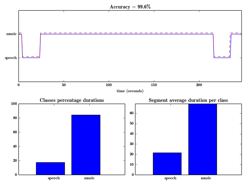
Note In the next section (hmm-based segmentation-classification) we present how both the fix-sized approach and the hmm approach can be evaluated using annotated datasets.
pyAudioAnalysis provides the ability to train and apply Hidden Markov Models (HMMs) in order to achieve joint classification-segmentation.
This is a supervised approach, therefore the required transition and prior matrices of the HMM model need to be trained.
Towards this end, function train_hmm_from_file() can be used to train a HMM model for segmentation-classification using a single annotated audio file.
A list of files stored in a particular folder can also be used, through calling function train_hmm_from_dir().
In both cases, an annotation file is needed for each audio recording (WAV file). HMM annotation files have a .segments extension (see above).
As soon as the model is trained, function hmm_segmentation() can be used to apply the HMM, in order to estimate the most probable sequence of class labels,
given a respective sequence of mid-term feature vectors. Note that hmm_segmentation() uses plot_segmentation_results() to plot results and evaluate the performance, as with the Fixed-segment Segmentation & Classification methodology.
Code example:
from pyAudioAnalysis import audioSegmentation as aS
aS.train_hmm_from_file('radioFinal/train/bbc4A.wav', 'radioFinal/train/bbc4A.segments', 'hmmTemp1', 1.0, 1.0)	# train using a single file
aS.train_hmm_from_dir('radioFinal/small/', 'hmmTemp2', 1.0, 1.0)							# train using a set of files in a folder
aS.hmm_segmentation('data/scottish.wav', 'hmmTemp1', True, 'data/scottish.segments')				# test 1
aS.hmm_segmentation('data/scottish.wav', 'hmmTemp2', True, 'data/scottish.segments')				# test 2
Command-line use examples:
python audioAnalysis.py trainHMMsegmenter_fromdir -i radioFinal/train/ -o data/hmmRadioSM -mw 1.0 -ms 1.0  (train)
python audioAnalysis.py segmentClassifyFileHMM -i data/scottish.wav --hmm data/hmmRadioSM                  (test)
It has to be noted that for shorter-term events (e.g. spoken words, etc), shorter mid-term windows need to be used when training the model. Try, for example the following example:
python audioAnalysis.py trainHMMsegmenter_fromfile -i data/count.wav --ground data/count.segments -o hmmcount -mw 0.1 -ms 0.1           (train)
python audioAnalysis.py segmentClassifyFileHMM -i data/count2.wav --hmm hmmcount                                         		(test)
Note 1 file hmmRadioSM contains a trained HMM model for speech-music discrimination.
It can be directly used for joint classification-segmentation of audio recordings, e.g.:
python audioAnalysis.py segmentClassifyFileHMM --hmm data/hmmRadioSM -i data/scottish.wav
Note 2
Function evaluate_segmentation_classification_dir() evaluates the performance of either a fixed-sized method or
an HMM model regarding the segmentation-classification task. This can also be achieved through the following command-line syntax:
python audioAnalysis.py segmentationEvaluation --model <method(svm, knn or hmm)> --modelName <modelName> -i <directoryName>
The first argument is either svm, knn or hmm. For the first two cases, the fix-sized segmentation-classification approach is used,
while for the third case the HMM approach is evaluated. In any case, the third argument must be the path of the file where the respective model is stored.
Finally, the third argument is the path of the folder where the audio files and annotations used in the evaluation process are stored.
Note that for each .wav file a .segments file (of the previously described three-column CSV format) must exist in the same folder.
If a .segments file does not exist for a particular audio file, then this is not computed in the final evaluation.
Execution examples:
python audioAnalysis.py segmentationEvaluation --model svm --modelName data/svmSM -i radioFinal/test/
python audioAnalysis.py segmentationEvaluation --model knn --modelName data/knnSM -i radioFinal/test/
python audioAnalysis.py segmentationEvaluation --model hmm --modelName data/hmmRadioSM -i radioFinal/test/
The result of these commands is the average segmentation-classification accuracy, along with the respective accuracies on each individual file of the provided folder.
Function silence_removal() from audioSegmentation.py takes an uninterrupted audio recording as input and returns segments endpoints
that correspond to individual audio events. In this way, all "silent" areas of the signal are removed.
This is achieved through a semi-supervised approach: first an SVM model is trained to distingush between high-energy and low-energy short-term frames. Towards this end, 10% of the highest energy frames along with the 10% of the lowest ones are used. Then, the SVM is applied (with a probabilistic output) on the whole recording and a dynamic thresholding is used to detect the active segments.
silence_removal() takes the following arguments: signal, sampling frequency, short-term window size and step,
window (in seconds) used to smooth the SVM probabilistic sequence, a factor between 0 and 1 that specifies how "strict" the thresholding is and finally a boolean associated to the ploting of the results. Usage Example:
from pyAudioAnalysis import audioBasicIO as aIO
from pyAudioAnalysis import audioSegmentation as aS
[Fs, x] = aIO.read_audio_file("data/recording1.wav")
segments = aS.silence_removal(x, Fs, 0.020, 0.020, smooth_window = 1.0, weight = 0.3, plot = True)
In this example, segments is a list of segments endpoints, i.e. each element is a list of two elements: segment beginning and segment end (in seconds).
A command-line call can be used to also generate WAV files with the detected segments. In the following example, a classification of all resulting segments using a predefined classifier (in our case speech vs music) is also performed:
python audioAnalysis.py silenceRemoval -i data/recording3.wav --smoothing 1.0 --weight 0.3
python audioAnalysis.py classifyFolder -i data/recording3_ --model svm --classifier data/svmSM --detail
The following figure shows the output of silence removal on file data/recording3.wav (vertical lines correspond to detected segment limits):
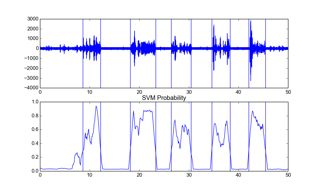
Depending on the nature of the recordings under study, different smoothing window lengths and probability weights must be used. The aforementioned examples,
where applied on two rather sparse recordings (i.e. the silent periods where quite long). For a continous speech recording (e.g. data/count2.wav) a
shorter smoothing window and a stricter probability threshold must be used, e.g.:
python audioAnalysis.py silenceRemoval -i data/count2.wav --smoothing 0.1 --weight 0.6
Speaker diarization is the task of automatically answering the question "who spoke when", given a speech recording. pyAudioAnalysis implements a variant of the speaker diarization method proposed in Giannakopoulos, Theodoros, and Sergios Petridis. "Fisher linear semi-discriminant analysis for speaker diarization." Audio, Speech, and Language Processing, IEEE Transactions on 20.7 (2012): 1913-1922..
In general, these are the main algorithmic steps performed by the implemented diarization approach:
- Feature extraction (short-term and mid-term). For each mid-term segment, the averages and standard deviations of the MFCCs are used, along with an estimate of the probabilities that the respective segment belongs to either a male or a female speaker (towards this end a trained model is used, named
knnSpeakerFemaleMale) - (optional) FLsD step: In this stage we obtain the near-optimal speaker discriminative projections of the mid-term feature statistic vectors using the FLsD approach.
- Clustering: A k-means clustering method is performed (either on the original feature space or the FLsD subspace). If the number of speakers is not a-priori known, the clustering process is repeated for a range of number of speakers and the Silhouette width criterion is used to find the optimal number of speakers.
- Smoothing: This step combines (a) a median filtering on the extracted cluster IDs and (b) a Viterbi Smoothing step.
Function speakerDiarization() from audioSegmentation.py can be used to extract a sequence of audio segments and respective cluster labels, given an audio file (see source code for documentation on arguments, etc).
In addition, function evaluateSpeakerDiarization() is used in speakerDiarization() in order to compare to sequences of cluster labels, one of which is the ground-truth, and thus to extract evaluation metrics.
In particular, the cluster purity and speaker purity are computed. Towards this end, a .segment ground-truth file is needed (with the same name with the WAV input file),
similarly to the general audio segmentation case. Finally, function speakerDiarizationEvaluateScript() can be used to extract the overall performance measures
for a set of audio recordings, and respective .segment files, stored in a directory.
Command-line example:
python audioAnalysis.py speakerDiarization -i data/diarizationExample.wav --num 4
This command takes the following arguments: -i <fileName>, --num <numberOfSpeakers (0 for unknown)>, --flsd (flag to enable FLsD method).
The result of this example is shown in the following figure (ground-truth is also illustrated in red). The performance measures are shown in the figure's title.
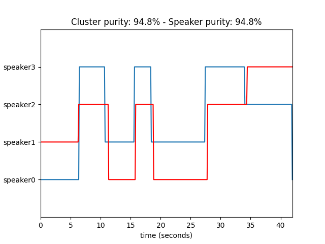
Note 1 The whole speaker diarization functionality can be applied in any task of clustering audio recordings.
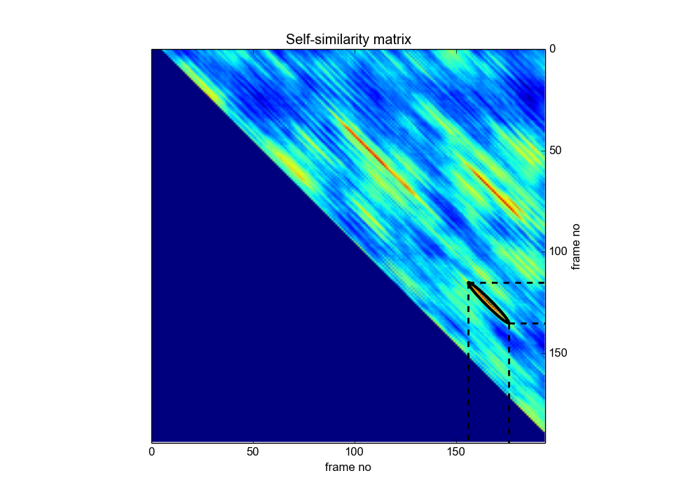
Audio thumbnailing is an important application of music information retrieval that focuses on detecting instances of the most
representative part of a music recording.
In pyAudioAnalysisLibrary this has been implemented in the musicThumbnailing(x, Fs, shortTermSize=1.0, shortTermStep=0.5, thumbnailSize=10.0)
function from the audioSegmentation.py.
The function uses the given wav file as an input music track and generates two thumbnails of <thumbnailDuration> length.
It results are written in two wav files <wavFileName>_thumb1.wav and <wavFileName>_thumb2.wav
It uses selfSimilarityMatrix() that calculates the self-similarity matrix of an audio signal (also located in audioSegmentation.py)
Command-line use:
python audioAnalysis.py thumbnail -i <wavFileName> --size <thumbnailDuration>
For example, the following thumbnail analysis is the result of applying the method on the famous song "Charmless Man" by Blur, using a 20-second thubmnail length. The automatically annotated diagonal segment represents the area where the self similarity is maximized, leading to the definition of the "most common segments" in the audio stream.