
Choose the Ideal Site for Designing Your Restaurant Using Data Science
Site analysis has a major role in placing a building, especially shopping malls,Shops, restaurant. Here we are trying to find some insights that help us to place our restaurant based on food type we are serving, characteristics of people who lives there, financial stability of people, demographic characteristics of the place, labor force etc.The analysis not only help owners to find ideal sites but also people to enjoy their favorite foods. Here the project tries to find locations of restaurants in Boston,is the capital and most populous city of the Commonwealth of Massachusetts in the United States.

- Datasets and Data-Loading
- Data Preprocessing
- Model creation
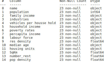
Data is collected from various channels and resources.Here we have used three major data sets .
GeoJSON is an open standard geospatial data interchange format that represents simple geographic features and their nonspatial attributes.
The Health Division of the Department of Inspectional Services (ISD) creates and enforces food safety codes to protect public health. All businesses which prepare and sell food to the public must possess a food service permit. In order to qualify for a permit, at least one full time employee must be must be certified through an accredited food manager program, which provides guidance on handling and serving food to the public.This dataset contains a list of restaurants that met the City's standards to become licensed food service establishments.
Boston in Context- Neighborhoods compares the United States, Massachusetts,Boston, and Boston’s neighborhoods across several social, economic, and housing characteristics. These data are from the 2014-2018 American Community Survey (ACS)
Preprocessing of data includes two steps
1)Removing unwanted columns and replace values
2)Scaling of features
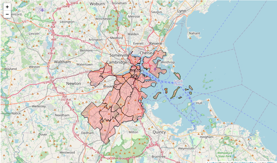
Visualizing the Boston map
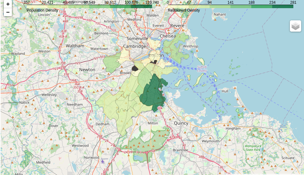
Visualizing the population density

Visualizing the restaurant locations
Model building has two parts:
1)K-Means Analysis
2)Principle Component Analysis
selected 6 clusters through elbow curve method.
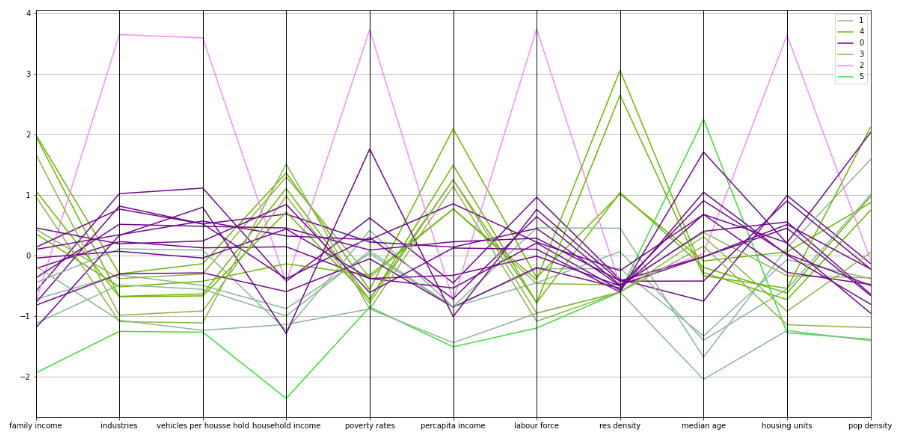
visualizing the clusters using parallel coordinate plot (ref: https://www.data-to-viz.com/graph/parallel.html.Parallel plot) or parallel coordinates plot allows to compare the feature of several individual observations (series) on a set of numeric variables. Each vertical bar represents a variable and often has its own scale. (The units can even be different). Values are then plotted as series of lines connected across each axis.
Parallel plots of clusters

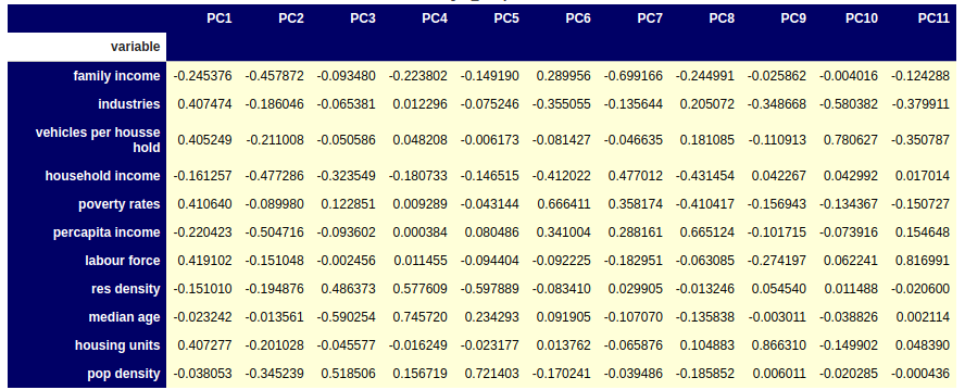
Eigen vector analysis :
Eigen value analysis:

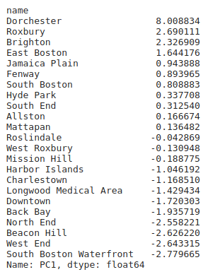
Principal component 1:

Places selected on basis of PC1:
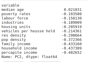
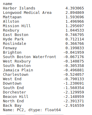
Principal component 2:
Places selected on basis of PC2:
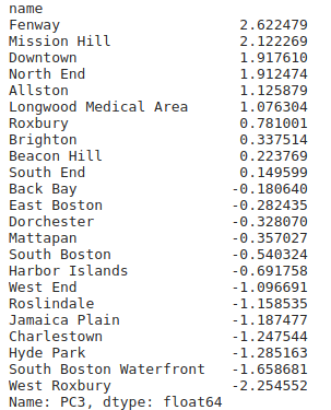
Principal component 3:

Places selected on basis of PC3:
Loading plot of PC1 and PC2 :

Bi-plot of PC1 and PC2 :

Below are the results got from Kmeans and PCA.
1,Cluster 2 has highest number of industries , vehicles,labor force , housing units,poverty rates
2,cluster 4 has highest percapita income and restaurant density
3,cluster 1 has lowest median age, Where youngsters are living
4,cluster 5 has lowest house hold income and highest median age.where old age people lives
PC1: This component is the measure of Labor force : 0.41 ,Healthcare: 0.40, Poverty rates: 0.40, industries: 0.40, housing units 0.40 and vehicles per house hold: .40 . Increase in PC1 tends to increases the correlating values. PC1 describes 47% of variance.
PC2: This component has can be measure of percapita income: -0.482,House hold income : -0.43 ,family income : 0.-43 and Population density:.37 . So, we can say PC2 tells about the Bad or worst. This suggest that when pc2 increases there will will be a low income.
PC3:This component affects the Population density : 48% and restaurant density :46% also negatively affects median age. This component may say that area in PC3 have young people so, restaurant density is high.The third principal component is a measure of the age and restaurant density.
The model is not finetuned .