For both methods, we will be attempting to path-plan in a planar-sphere world. The obstacles are circles inside of a circular workspace, which greatly simplifies the problem.
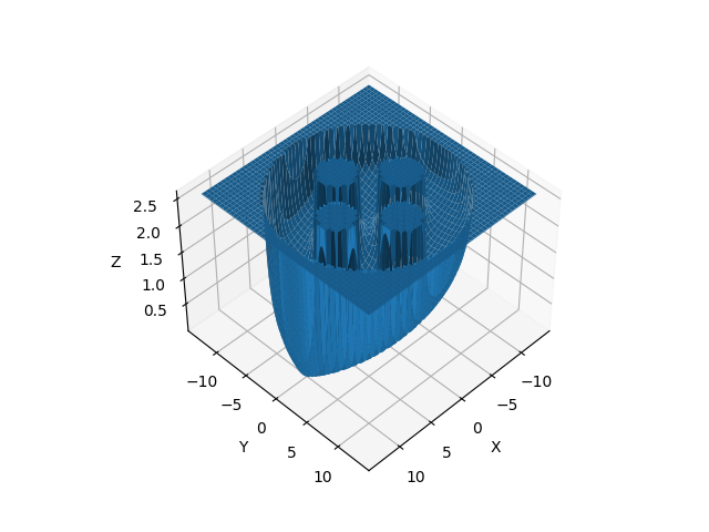
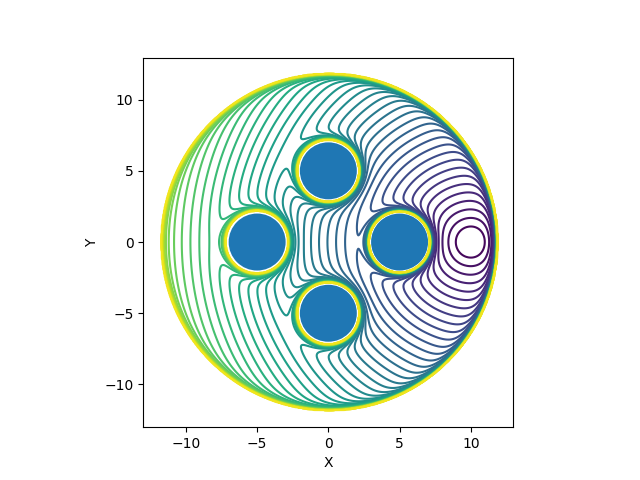
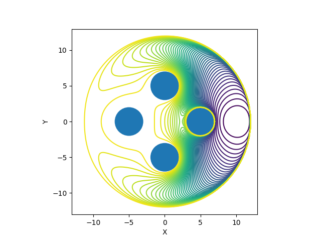
First, we will discuss path-planning using potential field methods. This uses the composition of an attractive potential and repulsive potential to create a potential function that has a global minimum at the goal position. The attractive potential is typically a quadratic function or the combination of a conic and quadratic function. In this case, we use the latter. Each obstacle in the space has a repulsive potential that is 0 when far from the obstacle and infinity at the obstacle's boundary. By composing these potential functions, we get a potential that is large near/in obstacles and follows the attractive potential everywhere else.
| Potential Surface | Potential Contours |
|---|---|
 |
 |
We can change how obstacles affect the potential by varying the parameter eta which effective scales the repulsive potential for each obstacle.
| Eta = 0.1 | Eta = 0.5 |
|---|---|
 |
 |
| Eta = 1 | Eta = 2 |
|---|---|
|
 |
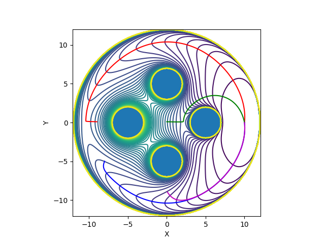
These potential functions are continuous and differentiable, so we can calculate a path using gradient descent. Since the global minimum of the attractive potential function is at the goal, in the presence of no obstacles we would always path-plan successfully to the goal. However, in the presence of obstacles, local minima arise that can cause gradient descent to get trapped so that it never reaches the goal.
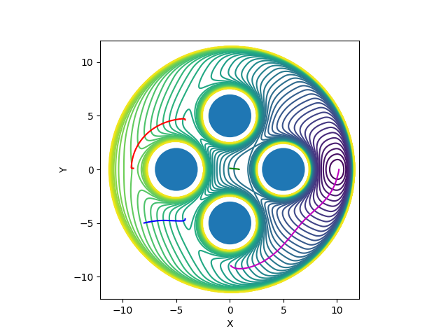
In this case, only one of the fours paths, purple, is able to avoid local minima and reach the goal. Navigation functions are able to solve this problem.
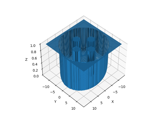
Navigation functions solve the problem of entrapment in local minima by removing them. On the surface level, the resulting surface looks very similar. However, navigation functions have attractive properties such as being smooth, continuous, and bounded to [0, 1]. Furthermore, they have unique global minimums that are isolated (i.e. they are Morse functions).
| Navigation Function Surface | Navigation Function Contours |
|---|---|
 |
 |
We can tune the shape of the navigation function by varying the parameter k. Increasing k flattens the navigation function at points close to and far away from the goal while making the transition areas steeper.
| K=3 | K=4 | K=5 |
|---|---|---|
|
 |
 |
We can use this function to path-plan using the same gradient descent algorithm as the potential-based planner. However, this time, there is a problem. As k gets larger, the areas we need to path-plan in have very small gradients. We can scale the gradient in our algorithm before taking a step, but we would need some intelligent scheme to scale it by a large value in the flat regions and a small value in the steep regions. Instead of doing this, we can scale the direction of the gradient by a fixed set step size. However, if this step size is too large to meet the tolerance for reaching the goal, we can overshoot. So, we also scale the gradient by a term in the range [0, 1] that decreases by an inverse square law from start to finish.
| 4 Paths K=3 | 4 Paths K=4 | 4 Paths K=5 |
|---|---|---|
 |
 |
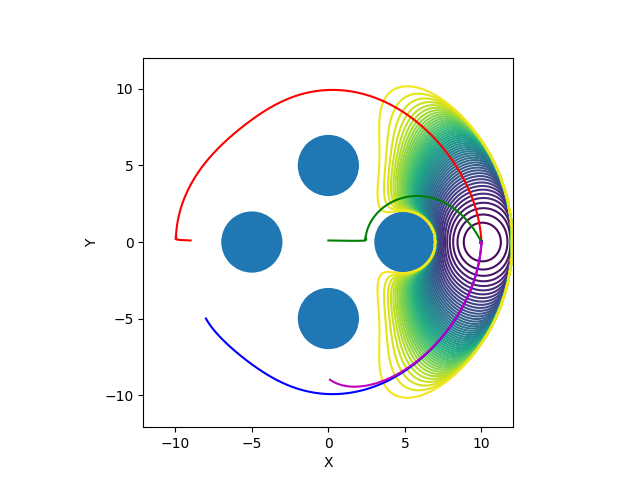 |
In each case, the planner successfully creates a path to the goal.
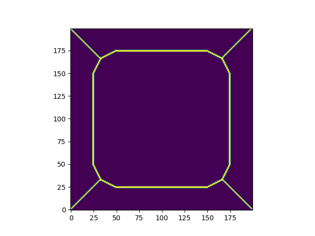
In the first three examples, we demonstrate the wave-front algorithm for generating the voronoi regions and the brushfire grid. The GVD is then simply created from the boundaries separating the Voronoi regions.
In the last example, we'll use the configuration of Example 3 to path-plan, using the GVD as a roadmap through the space.
Configuration: one square obstacle in the center of the workspace.
| Voronoi Region Generation | Brushfire Grid | Generalized Voronoi Diagram |
|---|---|---|
 |
 |
 |
Configuration: two triangular obstacles in opposite corners of the workspace.
| Voronoi Region Generation | Brushfire Grid | Generalized Voronoi Diagram |
|---|---|---|
 |
 |
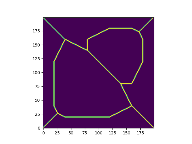 |
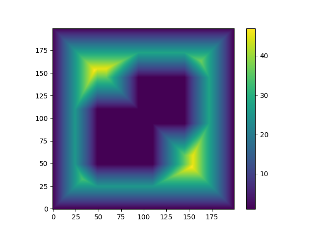
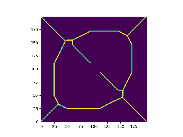
Configuration: two overlapping square obstacles.
| Voronoi Region Generation | Brushfire Grid | Generalized Voronoi Diagram |
|---|---|---|
 |
 |
 |
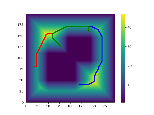
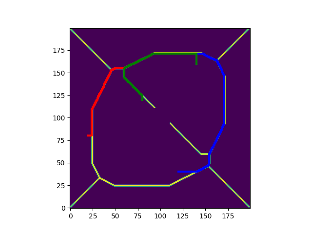
Task: path-plan to a goal from three points using the GVD in Example 3 as a roadmap.
| Path on Brushfire Grid | Path on GVD | Path in Real Space |
|---|---|---|
 |
 |
 |
This result demonstrates some important properties of the GVD in the brushfire grid:
-
Accessibility
- A trajectory can be made to reach a point on the roadmap from any point in the free space. In this implementation, this is done by following the path of steepest ascent in the brushfire potential from the goal until a point on the GVD is reached.
-
Connectivity
- Every point on the roadmap formed by the GVD is connected to every other point on the roadmap, so a trajectory can be made to reach any point on the roadmap from another.
-
Departability
- A trajectory can be made to reach a point in the free space from a point on the roadmap. In this implementation, this is done by following the path of steepest ascent in the brushfire potential from the goal until a point on the GVD is reached then reversing this path.