Kyphosis-Classification-Children-AfterSurgery

A study was conducted on children who had corrective spinal surgery. We are interested in factors that might result in kyphosis (a kind of deformation) after surgery.

data(kyphosis,package="rpart")

Consult the help page on the data for further details.

Make plots of the response as it relates to each of the three predictors. You may find a jittered scatterplot more effective than the interleaved histogram for a dataset of this size. Comment on how the predictors appear to be related to the response.

#Create the factor y to indicate the presence of Kyphosis
> kyphosis$y=ifelse(kyphosis$Kyphosis=="absent",0,1)

#Jittered scatterplot of Age
> ggplot(kyphosis, aes(x=Age, y= y)) + geom_point() + geom_jitter(width = 0.1, height = 0.1)

The predictor of Age might indicate a more likely occurrence of Kyphosis in the increase of the Age. But it is still uncertain.

#Jittered scatterplot of Number
> ggplot(kyphosis, aes(x=Number, y= y)) + geom_point() + geom_jitter(width = 0.1, height = 0.1)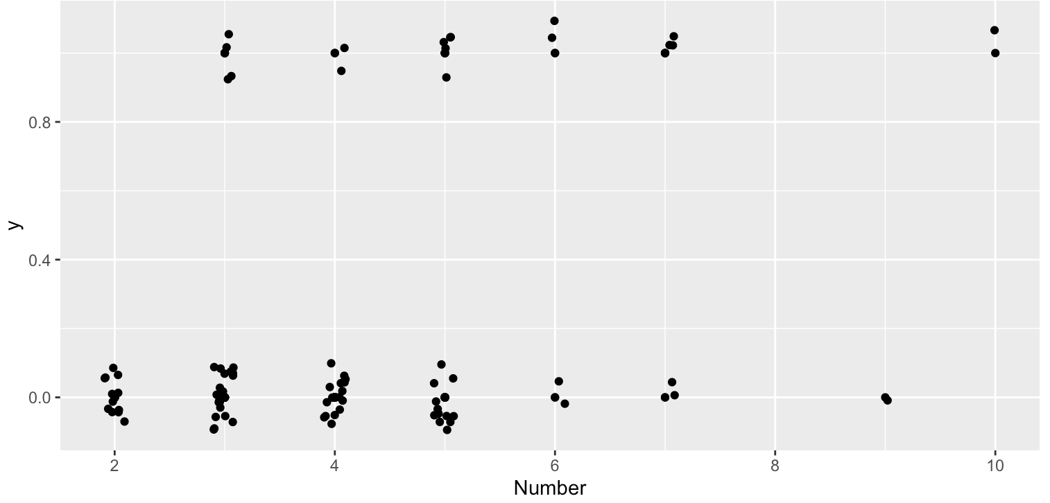

From this plot, as the increase of Number there might be more likely to have Kyphosis.

#Jittered scatterplot of Start
> ggplot(kyphosis, aes(x=Start, y= y)) + geom_point() + geom_jitter(width = 0.1, height = 0.1)

The plot shows that the lower values of Start might be more likely to have Kyphosis.

Fit a GLM with the kyphosis indicator as the response and the other three variables as predictors. Plot the deviance residuals against the fitted values.

#Fit the model 
> k1 <- glm(y~Age+Number+Start,data=kyphosis,family="binomial")
> summary(k1)

Call:
glm(formula = y ~ Age + Number + Start, family = "binomial", 
    data = kyphosis)

Deviance Residuals: 
    Min       1Q   Median       3Q      Max  
-2.3124  -0.5484  -0.3632  -0.1659   2.1613  

Coefficients:
             Estimate Std. Error z value Pr(>|z|)   
(Intercept) -2.036934   1.449575  -1.405  0.15996   
Age          0.010930   0.006446   1.696  0.08996 . 
Number       0.410601   0.224861   1.826  0.06785 . 
Start       -0.206510   0.067699  -3.050  0.00229 **
---
Signif. codes:  0 ‘***’ 0.001 ‘**’ 0.01 ‘*’ 0.05 ‘.’ 0.1 ‘ ’ 1

(Dispersion parameter for binomial family taken to be 1)

    Null deviance: 83.234  on 80  degrees of freedom
Residual deviance: 61.380  on 77  degrees of freedom
AIC: 69.38

Number of Fisher Scoring iterations: 5

#Plot the deviance residuals against the fitted values
> linpred=predict(k1)
> predprob=predict(k1,type='response')
> head(linpred)
          1           2           3           4           5           6 
-1.06161598 -1.96925448 -0.02797731 -0.16857667 -3.48124904 -4.50896146 
> head(predprob)
         1          2          3          4          5          6 
0.25700076 0.12246899 0.49300613 0.45795535 0.02985049 0.01088999 
> head(ilogit(linpred))
         1          2          3          4          5          6 
0.25700076 0.12246899 0.49300613 0.45795535 0.02985049 0.01088999 
> rawres=kyphosis$y-predprob
> plot(rawres~linpred,xlab='Linear Predictor',ylab='Residuals')

This plot cannot provide useful information.

Produce a binned residual plot as described in the text. Comment on the plot.

# better way to display residuals - first group into bins, then plot bin averages
> library(dplyr)
> kyphosis=mutate(kyphosis,residuals=residuals(k1),linpred=predict(k1))
> gdf=group_by(kyphosis,cut(linpred,breaks=unique(quantile(linpred,(0:12)/12))))
> diagdf=summarise(gdf,residuals=mean(residuals),linpred=mean(linpred))
> plot(residuals~linpred,diagdf,xlab='Linear Predictor',pch=20)

We group them into 12 bins and then plot bin averages. Now, the plot can provide more useful Information. It is roughly a random scatter plot which indicates good enough fitting.

Plot the residuals against the Start predictor, using binning as appropriate. Comment on the plot.

#Plot the residuals against the Start predictor
> gdf=group_by(kyphosis,Start)
> diagdf=summarise(gdf,residuals=mean(residuals))
> ggplot(diagdf,aes(x=Start,y=residuals))+geom_point()

The plot is randomly scattered and it meets our expectations. It fits the model well.

Produce a normal QQ plot for the residuals. Interpret the plot.

# QQ-plot for the residuals 
> qqnorm(residuals(k1))

The plot is not a prefect straight-line. It is good to know that we don't expect lineaer relationship with binary data.

Make a plot of the leverages. Interpret the plot.

# The leverages plot
> halfnorm(hatvalues(k1))

There is no obvious influential outliers. Although the obs53 and obs24 are labeled, they still fit the line farily well.

Check the goodness of fit for this model. Compute the Hosmer-Lemeshow statistic and associated p-value. What do you conclude?

> kyphosisM=mutate(kyphosis,predprob=predict(k1,type='response'))
> gdf=group_by(kyphosisM,cut(linpred,breaks=unique(quantile(linpred,(0:12)/12))))
> hldf=summarise(gdf,y=sum(y),ppred=mean(predprob),count=n())
> hldf=mutate(hldf,se.fit=sqrt(ppred*(1-ppred)/count))
# Plot
> ggplot(hldf,aes(x=ppred,y=y/count,ymin=y/count-2*se.fit,ymax=y/count+2*se.fit))+geom_point()+
geom_linerange(color=grey(0.75))+geom_abline(intercept=0,slope=1)+xlab('Predicted Probability')+ylab("Observed Proportion")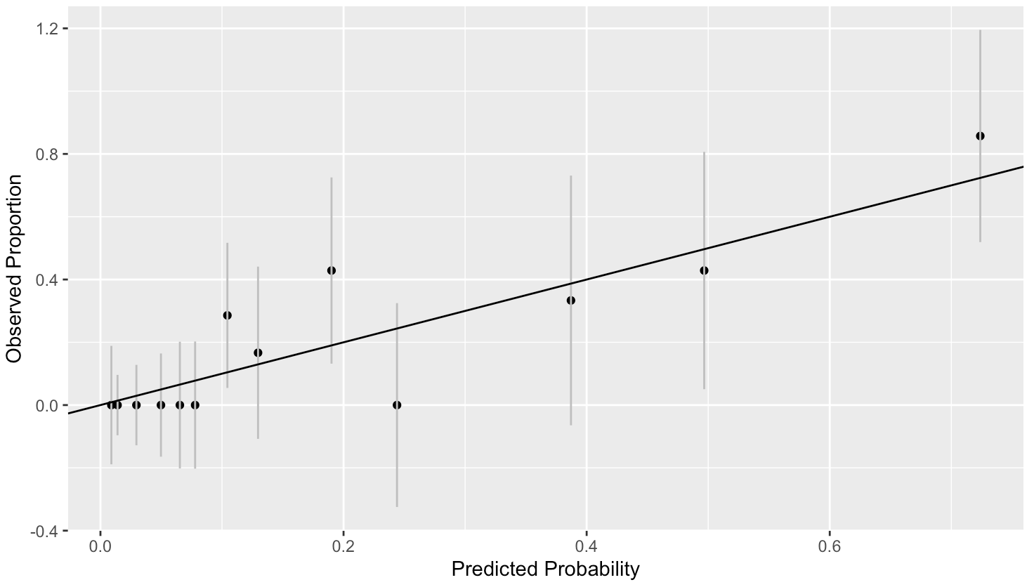

# Compute the Hosmer-Lemeshow statistic and associated p-value
> hlstat=with(hldf,sum((y-count*ppred)^2/(count*ppred*(1-ppred))))
> c(hlstat,nrow(hldf)) 
[1]  9.887868 13.000000
> 1-pchisq(9.887868,13-1)
[1] 0.6257974

Although we can see there is some variation in the plot, there is no consistent deviation from what is expected. We have computed approximate 95% confidence intervals using the binomial variation. The line passes through all of these intervals confirming that the variation from the expected is not excessive.

The p-value = 0.6257974 which is very high. Thus, we detect no lack of fit.

Use the model to classify the subjects into predicted outcomes using a 0.5 cutoff. Produce cross-tabulation of these predicted outcomes with the actual outcomes. When kyphosis is actually present, what is the probability that this model would predict a present outcome?

> kyphosisM <- mutate(kyphosisM, predout=ifelse(predprob < 0.5, "no", "yes"))
> xtabs( ~ y + predout, kyphosisM)
   predout
y   no yes
  0 61   3
  1 10   7

We see how the classifications match with the observed outcomes. The correct classification rate is:

> (61+7)/(61+7+10+3)
[1] 0.8395062

The correct classification rate is 84%.

The proportion of those who will develop kyphosis that are correctly identified by the model is called the sensitivity.

> 7/(10+7)
[1] 0.4117647

The sensitivity is about 41%.