scikit-eo: A Python package for Remote Sensing Data Analysis

Introduction

Nowadays, remotely sensed data has increased dramatically. Microwaves and optical images with different spatial and temporal resolutions are available and are used to monitor a variety of environmental issues such as deforestation, land degradation, land use and land cover change, among others. Although there are efforts (i.e., Python packages, forums, communities, etc.) to make available line-of-code tools for pre-processing, processing and analysis of satellite imagery, there is still a gap that needs to be filled. In other words, too much time is still spent by many users developing Python lines of code. Algorithms for mapping land degradation through a linear trend of vegetation indices, fusion optical and radar images to classify vegetation cover, and calibration of machine learning algorithms, among others, are not available yet.

Therefore, scikit-eo is a Python package that provides tools for remote sensing. This package was developed to fill the gaps in remotely sensed data processing tools. Most of the tools are based on scientific publications, and others are useful algorithms that will allow processing to be done in a few lines of code. With these tools, the user will be able to invest time in analyzing the results of their data and not spend time on elaborating lines of code, which can sometimes be stressful.

Tools for Remote Sensing

Name of functions/classes	Description
mla	Machine Learning (Random Forest, Support Vector Machine, Decition Tree, Naive Bayes, Neural Network, etc.)
calmla	Calibrating supervised classification in Remote Sensing (e.g., Monte Carlo Cross-Validation, Leave-One-Out Cross-Validation, etc.)
confintervalML	Information of confusion matrix by proportions of area, overall accuracy, user's accuracy with confidence interval and estimated area with confidence interval as well.
rkmeans	K-means classification
calkmeans	This function allows to calibrate the kmeans algorithm. It is possible to obtain the best k value and the best embedded algorithm in kmeans.
pca	Principal Components Analysis
atmosCorr	Atmospheric Correction of satellite imagery
deepLearning	Deep Learning algorithms
linearTrend	Linear trend is useful for mapping forest degradation or land degradation
fusionrs	This algorithm allows to fuse images coming from different spectral sensors (e.g., optical-optical, optical and SAR or SAR-SAR). Among many of the qualities of this function, it is possible to obtain the contribution (%) of each variable in the fused image
sma	Spectral Mixture Analysis - Classification sup-pixel
tassCap	The Tasseled-Cap Transformation

You will find more algorithms!.

Installation

To use scikit-eo it is necessary to install it. There are two options:

1. From PyPI

scikit-eo is available on PyPI, so to install it, run this command in your terminal:

pip install scikeo

2. Installing from source

It is also possible to install the latest development version directly from the GitHub repository with:

pip install git+https://github.com/ytarazona/scikit-eo

Example

1.0 Applying Machine Learning

Libraries to be used:

import rasterio
import numpy as np
from scikeo.mla import MLA
import matplotlib.pyplot as plt
from dbfread import DBF
import matplotlib as mpl
import pandas as pd

2.0 Optical image

Landsat-8 OLI (Operational Land Imager) will be used to obtain in order to classify using Random Forest (RF). This image, which is in surface reflectance with bands:

• Blue -> B2
• Green -> B3
• Red -> B4
• Nir -> B5
• Swir1 -> B6
• Swir2 -> B7

The image and signatures to be used can be downloaded here:

3.0 Supervised Classification using Random Forest

Image and endmembers

path_raster = r"C:\data\ml\LC08_232066_20190727_SR.tif"
img = rasterio.open(path_raster)

path_endm = r"C:\data\ml\endmembers.dbf"
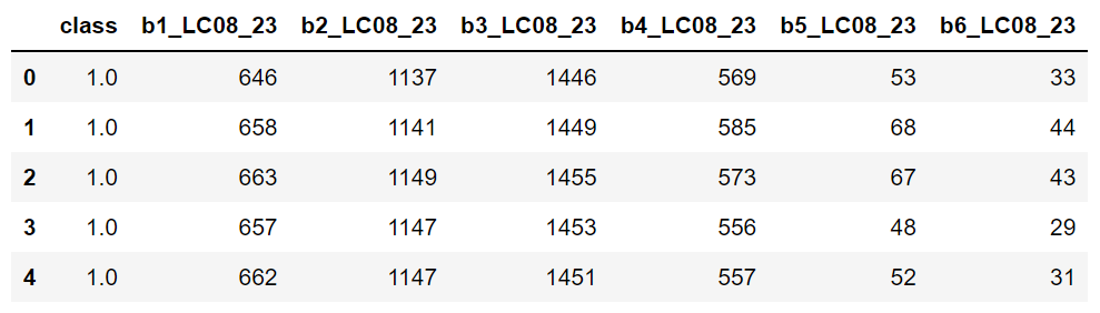
endm = DBF(path_endm)

# endmembers
df = pd.DataFrame(iter(endm))
df.head()

Instance of mla():

inst = MLA(image = img, endmembers = endm)

Applying Random Forest:

svm_class = inst.SVM(training_split = 0.7)

4.0 Results

Dictionary of results

svm_class.keys()

Overall accuracy

svm_class.get('Overall_Accuracy')

Kappa index

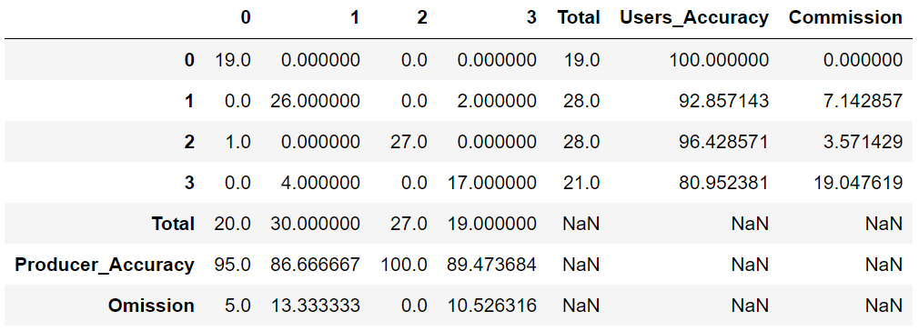
svm_class.get('Kappa_Index')

Confusion matrix or error matrix

svm_class.get('Confusion_Matrix')

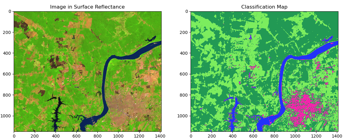
Preparing the image before plotting

# Let's define the color palette
palette = mpl.colors.ListedColormap(["#2232F9","#F922AE","#229954","#7CED5E"])

Applying the plotRGB() algorithm is easy:

# Let´s plot
fig, axes = plt.subplots(nrows = 1, ncols = 2, figsize = (15, 9))

# satellite image
plotRGB(img, title = 'Image in Surface Reflectance', ax = axes[0])

# class results
axes[1].imshow(svm_class.get('Classification_Map'), cmap = palette)
axes[1].set_title("Classification map")
axes[1].grid(False)

• Free software: Apache Software License 2.0
• Documentation:

Acknowledgment

Special thanks to:

• David Montero Loaiza for the idea of the package name scikit-eo.

• Qiusheng Wu for the suggestions that helped to improve the package.

Credits

This package was created with Cookiecutter