Software Requirements Analysis Specification Document
Revision History
| Date | Version | Description |
|---|---|---|
| <12/20/2019> | <1.0> | First Draft of the Software Requirement Analysis Specification Doc. |
- Software Requirements Analysis Specification Document
The Software Requirements Analysis Specification is designed to document and describe the agreement between the software user and the developer regarding the specification of the software product requested. Its primary purpose is to provide a clear and descriptive “statement of user requirements” that can be used as a reference in the further development of the software system. This document is broken into a number of sections used to logically separate the software requirements into easily referenced parts.
This Software Requirements Analysis Specification aims to describe the functionality, external interfaces, attributes and design constraints imposed on the Implementation of the software system described throughout the rest of the document. Throughout the description of the software system, the language and terminology used should be unambiguous and consistent throughout the document.
This document provides an architectural overview of the Sage Linear System Solver, which is a set of several GPU-accelerated algorithms for linear systems. The primary purpose of the software is to accelerate the iterative solutions for large sparse linear systems using NVIDIA CUDA parallel computing architecture platform and making full use of GPU computing resources.
This document is intended to capture and convey the significant architectural decisions which have been made in designing and building the system. It is a way by which the systems’ architect and others involved in the project can better understand the problems to be solved and how it will be represented with this system.
This project focuses on the research and program development of solving linear equations from FEA (Finite Element Analysis) drawing on expertise from School of Software Engineering and College of Civil Engineering.
FEA (Finite Element Analysis) uses mathematical approximation to simulate real physical systems such as geometry and load conditions. With simple and interacting elements or units, a finite number of unknowns can be used to approximate an infinite unknowns in real system.
With the development of computer technology, the amount of computer storage is increasing, and the calculation speed is rapidly increasing. However, the scale of the problems to be solved is getting larger and larger, and the requirements for calculation storage and speed are becoming higher and higher. For example, there are hundreds of millions or more of unknown linear equations from problems such as finite element analysis of bridge structural mechanics and atmospheric prediction. In the field of Civil Engineering, the problems of concrete static analysis and bridge structure analysis of structural engineering, tunnel excavation in geotechnical engineering, rock blasting, artificial islands and access roads, and analysis of settlement of large oil storage tanks can all be concluded. Therefore, constructing efficient methods for solving discrete equations is an important part of computational mathematics for solving the finite element linear equations. At present, there are mainly two methods — direct solution method and iterative method.
For large matrices, the direct solution method requires a large amount of memory, and the amount of calculation is also very large. It usually takes several days or even months. Therefore, in practical applications, the iterative method is currently the main method for solving large-scale linear equations. It can make full use of the properties of the coefficient matrix including less memory occupation, easy calculation and simple program. In the basic iterative solution of linear equations, we mainly study how various basic iterative methods establish iterative schemes, prove iterative convergence conditions, adopt error estimates, and evaluate convergence speed.
In order to improve the calculation efficiency and shorten the calculation time, we also tried to use CUDA ™ (Compute Unified Device Architecture), a universal parallel computing architecture platform launched by NVIDIA®, to accelerate the solving of linear equations by using the idea of GPU parallel computing.
CUDA® is a parallel computing platform and programming model developed by NVIDIA for general computing on graphical processing units (GPUs). With CUDA, developers are able to dramatically speed up computing applications by harnessing the power of GPUs.
In GPU-accelerated applications, the sequential part of the workload runs on the CPU – which is optimized for single-threaded performance – while the compute intensive portion of the application runs on thousands of GPU cores in parallel. When using CUDA, developers program in popular languages such as C, C++, Fortran, Python and MATLAB and express parallelism through extensions in the form of a few basic keywords.
For the further use of hardware acceleration algorithms, we explored the feasibility of GPU-accelerated deployment in Kubernetes to isolate GPU computing services and automatically load balance multi-GPU tasks.
Kubernetes is an open source system for managing containerized applications across multiple hosts. It provides basic mechanisms for deployment, maintenance, and scaling of applications.
Kubernetes builds upon a decade and a half of experience at Google running production workloads at scale using a system called Borg, combined with best-of-breed ideas and practices from the community.
Table of Glossary
| Terms | Definition |
|---|---|
| FEA | Finite Element Analysis |
| SLSS | Sage Linear System Solver |
| CUDA | Compute Unified Device Architecture, a parallel computing platform and programming model developed by NVIDIA. |
| Kubernetes | An open source system for managing containerized applications across multiple hosts. |
| Linear System | A linear system is a mathematical model of a system based on the use of a linear operator. |
| Linear Equation | A linear equation in two variables describes a relationship in which the value of one of the variables depends on the value of the other variable. |
| Iterative Method | In computational mathematics, an iterative method is a mathematical procedure that uses an initial guess to generate a sequence of improving approximate solutions for a class of problems, in which the n-th approximation is derived from the previous ones. |
| Jacobi Method | In numerical linear algebra, the Jacobi method is an iterative algorithm for determining the solutions of a strictly diagonally dominant system of linear equations. |
| SOR Method | In numerical linear algebra, the method of successive over-relaxation (SOR) is a variant of the Gauss–Seidel method for solving a linear system of equations, resulting in faster convergence. |
| Gauss-Seidel Method | In numerical linear algebra, the Gauss–Seidel method, also known as the Liebmann method or the method of successive displacement, is an iterative method used to solve a linear system of equations. |
| Conjugate Gradient Method | In mathematics, the conjugate gradient method is an algorithm for the numerical solution of particular systems of linear equations, namely those whose matrix is symmetric and positive-definite. |
| Positive-definite Matrix | In linear algebra, a symmetric |
| Diagonally Dominant Matrix | In mathematics, a square matrix is said to be diagonally dominant if, for every row of the matrix, the magnitude of the diagonal entry in a row is larger than or equal to the sum of the magnitudes of all the other (non-diagonal) entries in that row. |
| CSR Format | Compressed Sparse Row Format (CSR), represents a matrix M by three (one-dimensional) arrays. |
| Host | In CUDA, the host refers to the CPU and its memory |
| Device | In CUDA, the device refers to the GPU and its memory. |
| Kernel | Functions executed on the device, which are executed by many GPU threads in parallel |
This document is intended for all individuals participating in and supervising the Sage Linear System Solver Project, which is essentially a sub-topic of a scientific research topic. At the same time, it is a Software Engineering course project. Thus, its intended audience are mainly teachers from the College of Civil Engineering as well as the instructors of the Software Engineering course.
All readers are strongly recommended to read the first section of the document, which introduces the project scope, background knowledge, and some terms used in the document.
The second section is recommended as well for all readers, which systematically introduces the functional requirements involved in the project at a high level. In this section, a detailed system scope will be provided, and the architecture and the flow of the entire system will be analyzed and illustrated in the form of pictures and text.
Readers who wants to learn more details about the nonfunctional requirements regarding to the system are recommended to read the third section, which includes additional specification such as performance, safety, security and software quality requirements which does not fit into other sections.
If readers want to know the regulations regarding the operating environment of the system, they may find answers in the fourth section.
- IEEE-SA Standards Board. IEEE Std 830-1998 IEEE Recommended Practice for Software Requirements Specifications. Software Engineering Standards Committee of the IEEE Computer Society, June 25 th 1998.
- Craig Larman. Applying UML and Patterns: An Introduction to Object-Oriented Analysis and Design and Iterative Development, Third Edition. Addison Wesley Professional, October
$20^{\text{th}}$ 2004 - Doug Rosenberg, Matt Stephens. Use Case Driven Object Modeling with UML: Theory and Practice. Apress, 2007.
- Roger S. Pressman, Bruce R. Maxim. Software Engineering: A Practitioner's Approach, Eighth Edition. McGraw-Hill Education, 2005.
The software system is called Sage Linear System Solver or SLSS. It is produced primarily for people who have strong demands for fast solutions for large linear systems including but not limited to the civil engineering practitioners, structural engineer, and students and instructors in related major, etc.
This system is designed to provide automation support for the process of solving all kinds of linear systems which can be uploaded by the users. As long as the uploaded matrices can meet certain constraints (Say they are symmetric positive definite matrices, or strictly diagonally dominant matrices), the system can output the solution vector when the result is convergent. This system provides four different algorithms (both stationary iterative methods and non-stationary iterative methods) and up to more than ten calculation interfaces to solve linear equations. Users can select one or several algorithms at one time, in order to compare the efficiency of different algorithms or the efficiency of CPU execution and GPU execution. Users can also view the analysis of different methods in the form of line charts and bar charts, including how much time it takes respectively and how many iterations it takes to make it convergent. In addition, users can download the solution vectors for further computation.
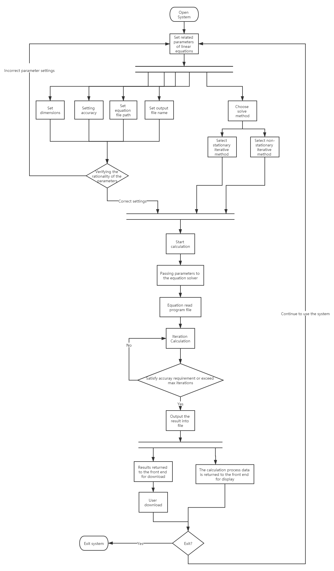
Activity Diagram of Initializing Solver Use Case
Activity Diagram of Viewing Results Use Case
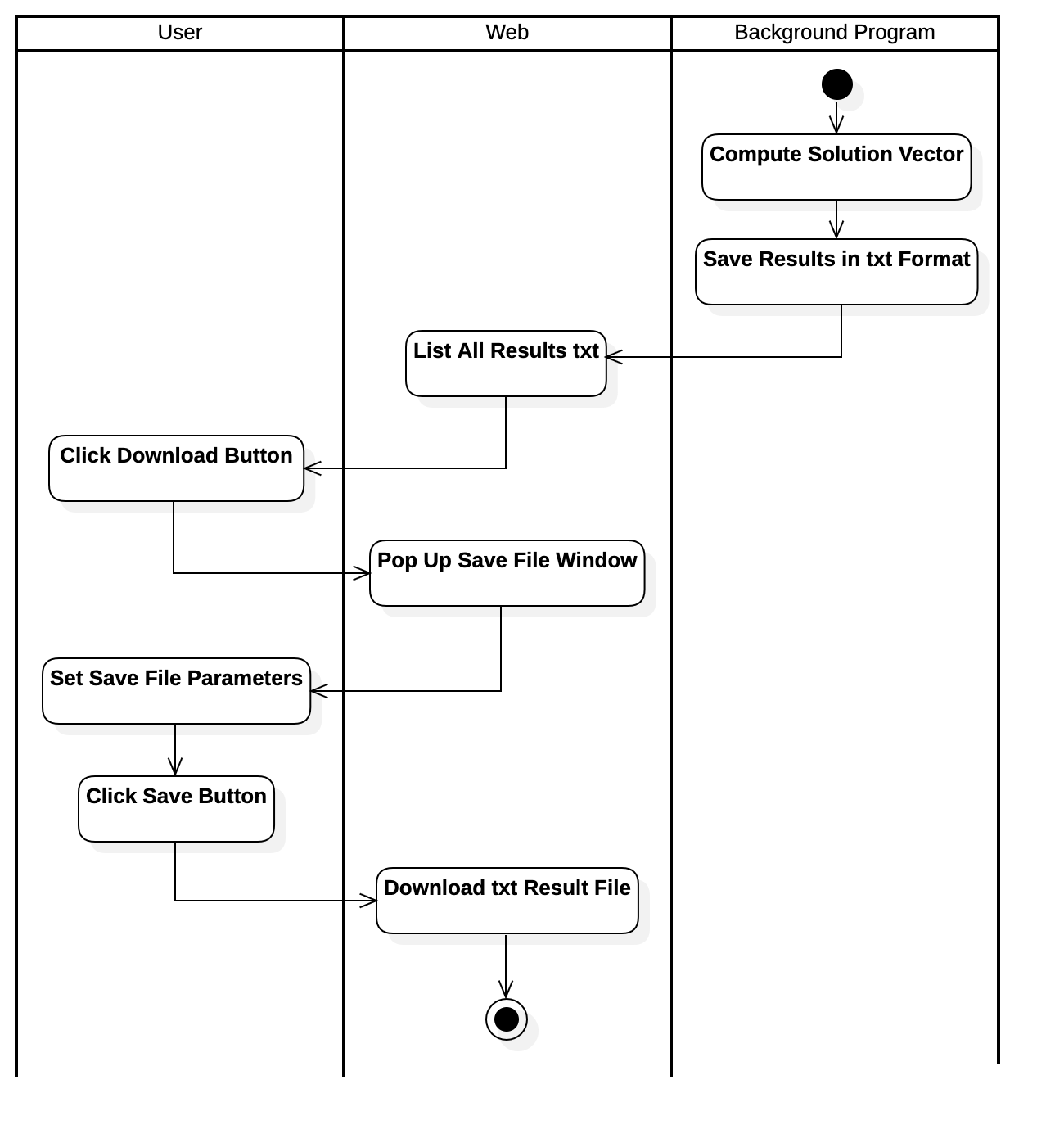
Activity Diagram of Downloading Results Use Case
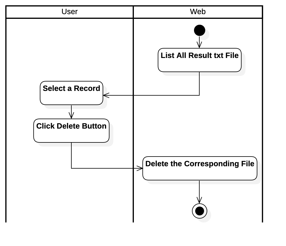
Activity Diagram of Deleting Results Parameters Use Case
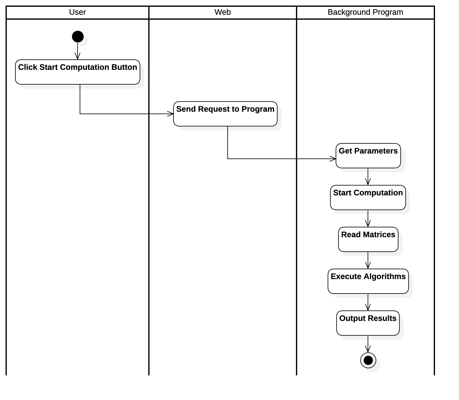
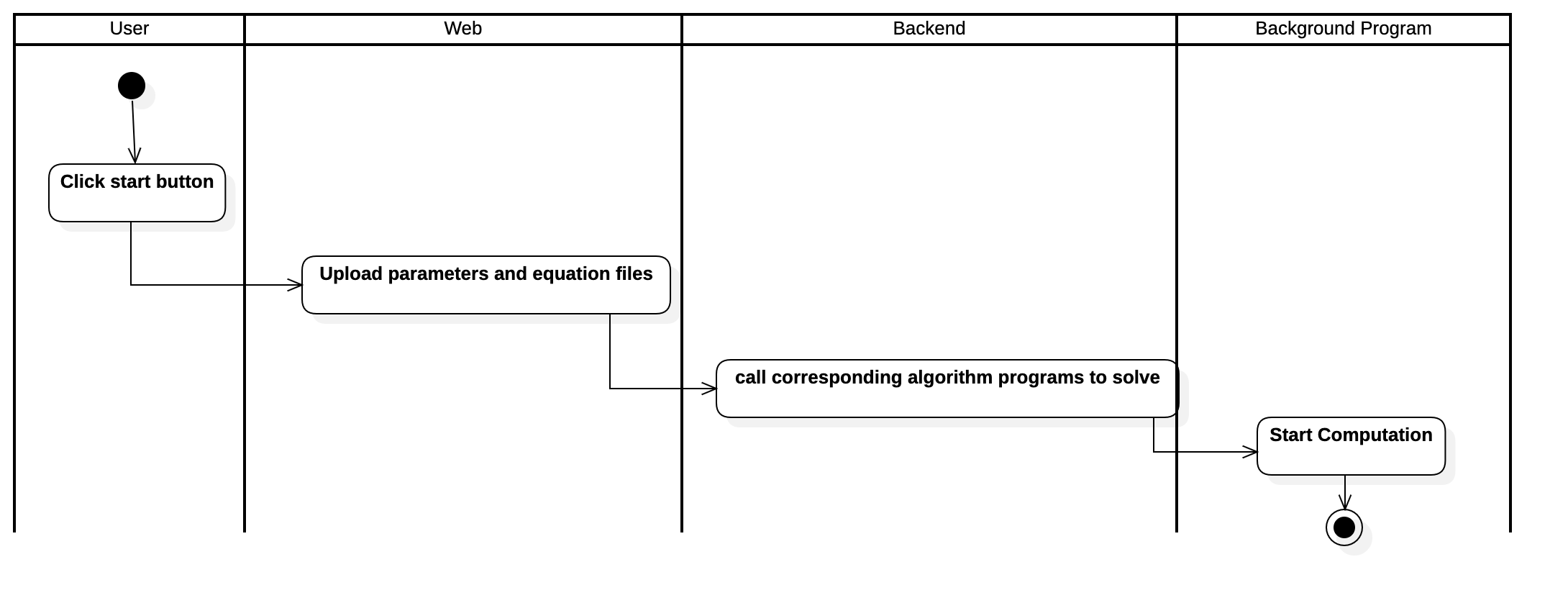
Activity Diagram of Computing Results Use Case
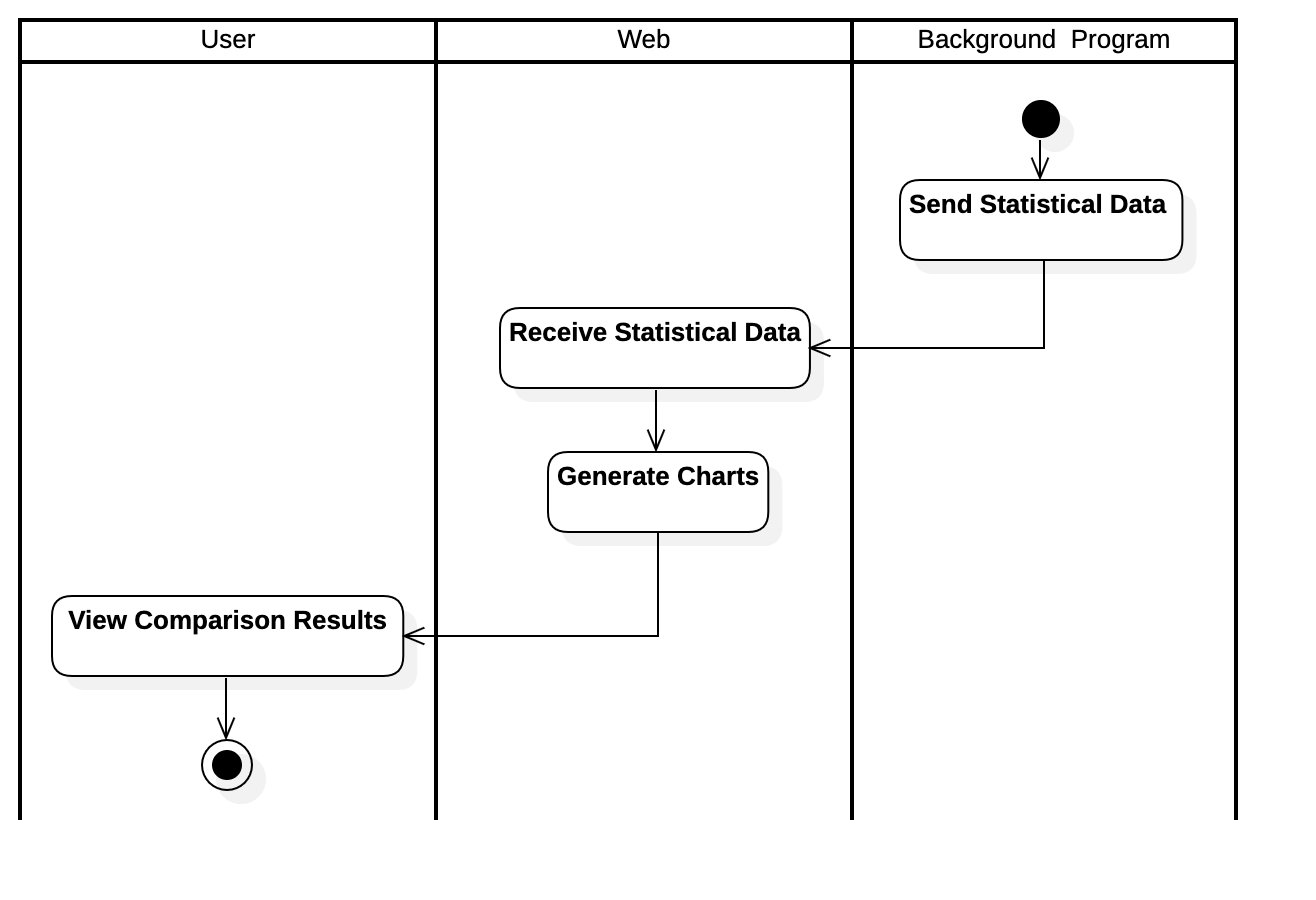
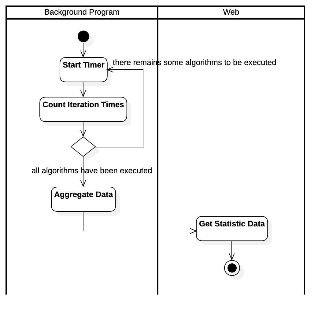
Activity Diagram of Analyzing Results Use Case
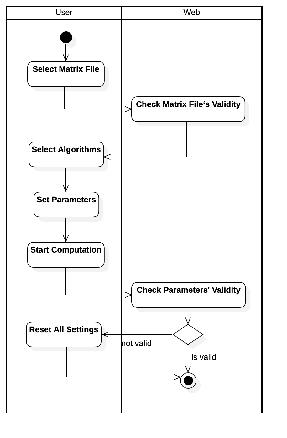
Activity Diagram of Selecting Matrix Files Use Case
Activity Diagram of Selecting Algorithms Use Case
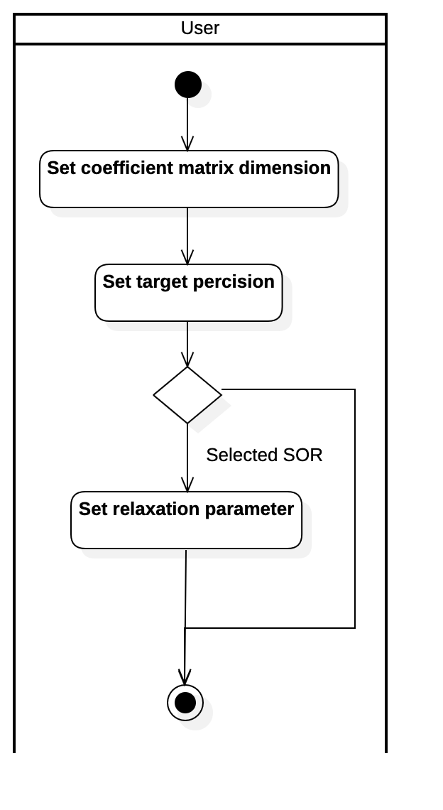
Activity Diagram of Setting Parameters Use Case
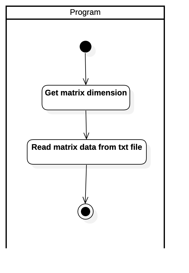
Activity Diagram of Reading Matrix Data Use Case
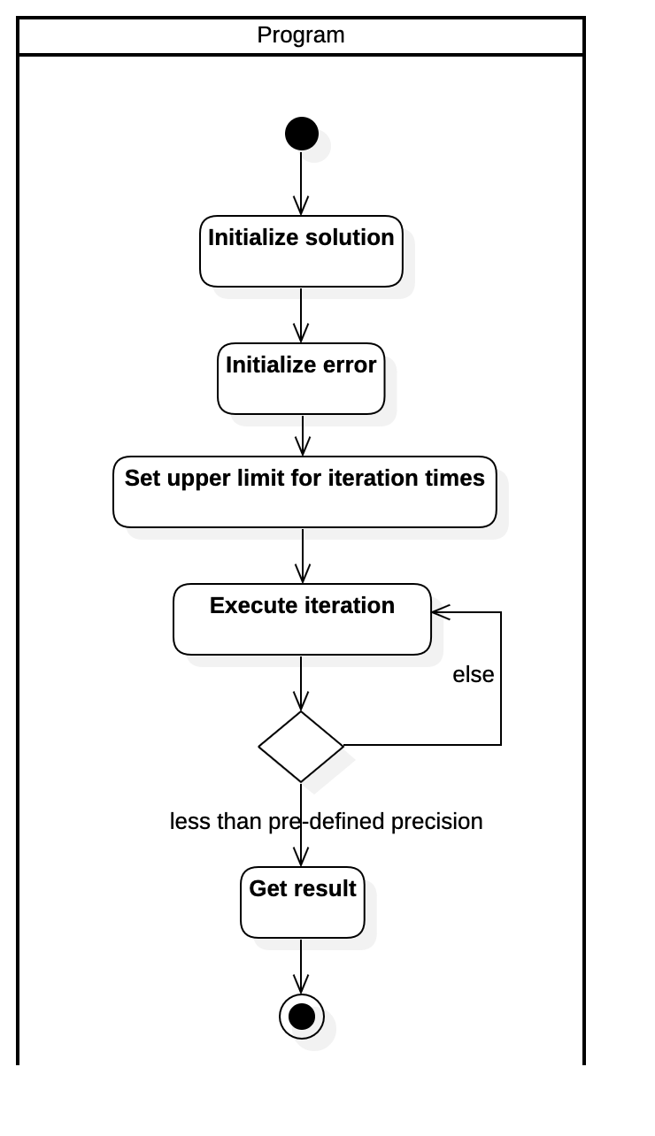
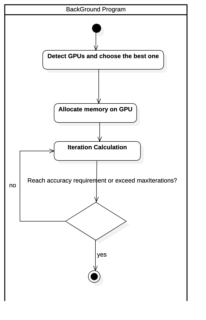
Activity Diagram of Executing Algorithms Use Case
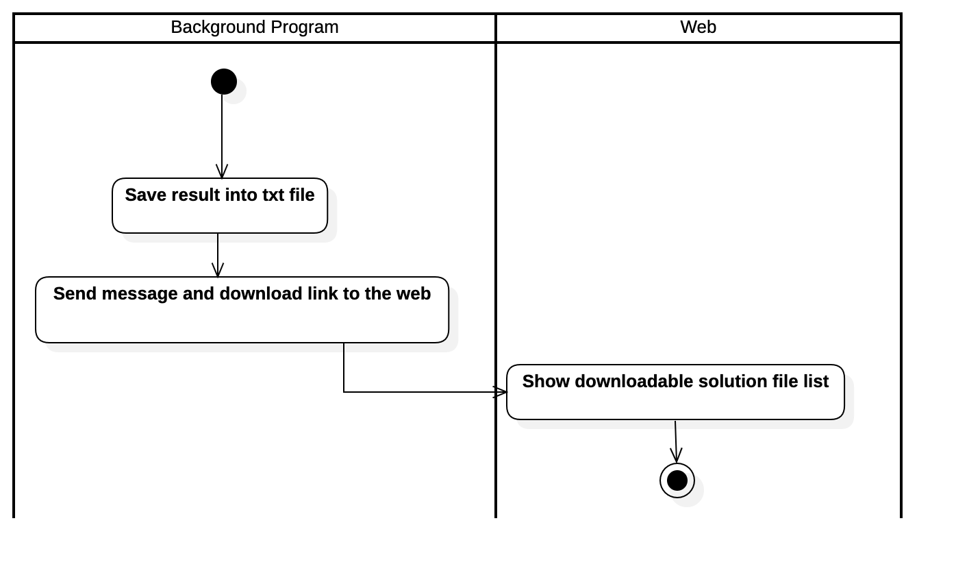
Activity Diagram of Outputting Results Use Case
Activity Diagram of Uploading Matrix Files Use Case
Activity Diagram of Executing Gauss-Seidel Iteration Use Case
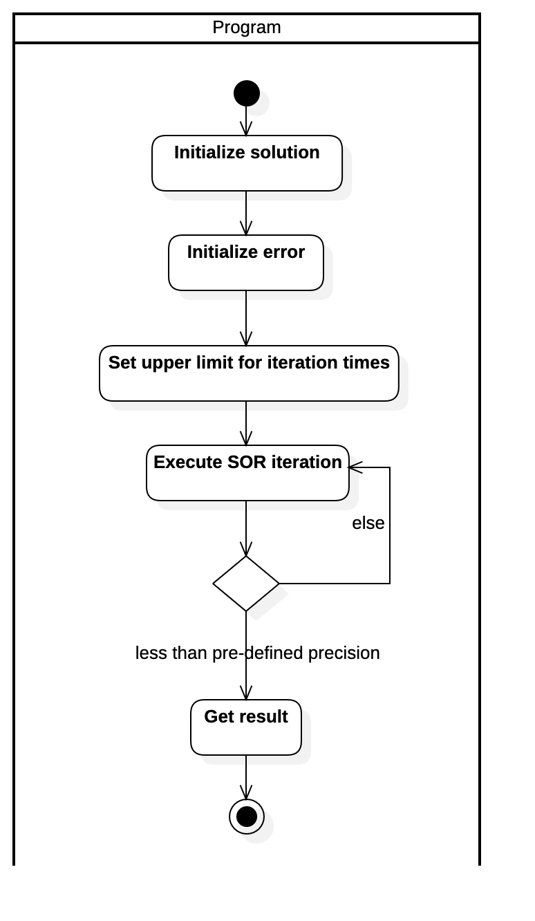
Activity Diagram of Executing SOR Iteration Use Case
Activity Diagram of Executing Jacobi Iteration Use Case
Activity Diagram of Executing Conjugate Gradient Iteration Use Case
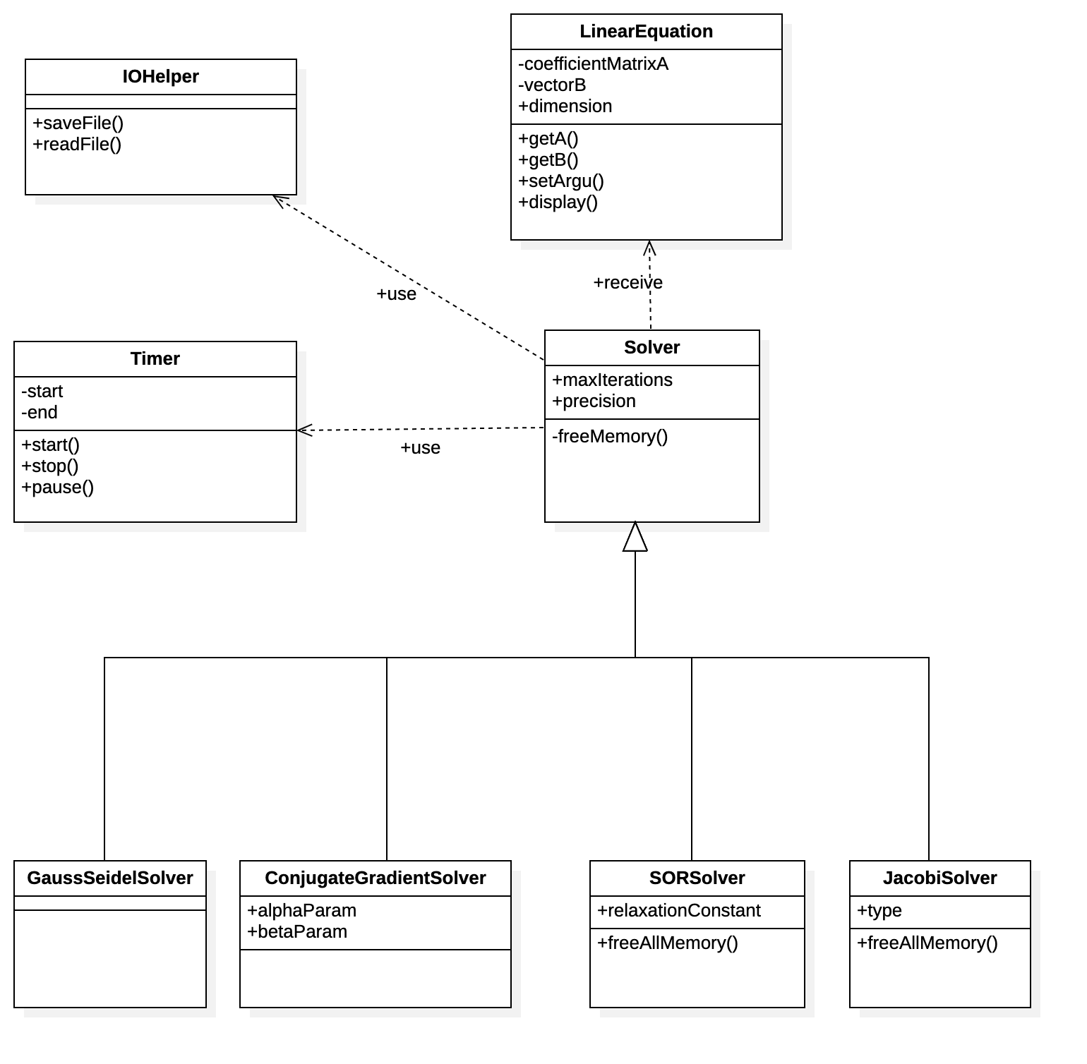
The following diagram is the analysis class diagram.
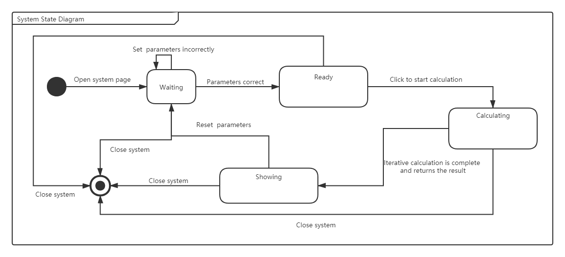
The following diagram describes the migration of the entire systems' states.
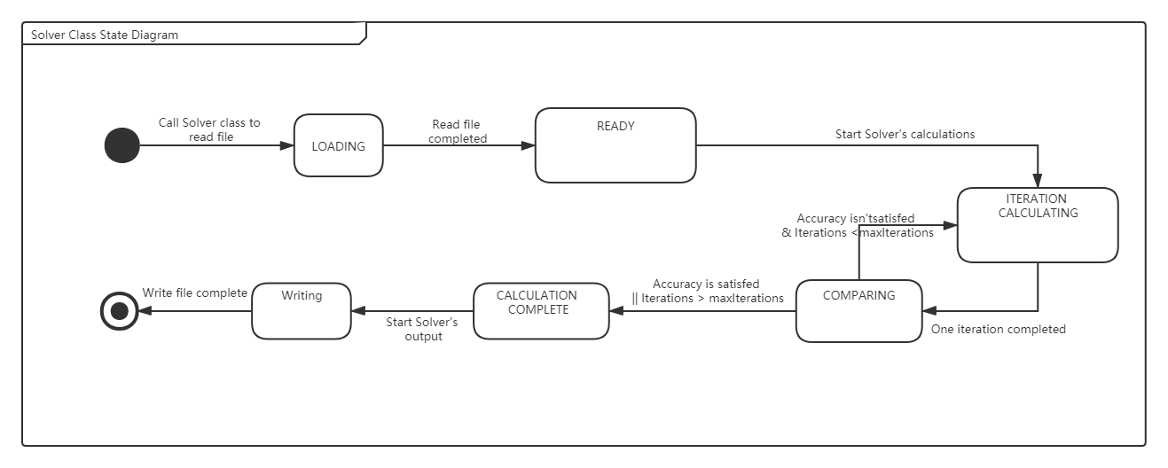
The following diagram illustrates the migration of the states of the solver class.
Since the front-end interface is not the focus of our work, we will mainly discuss the static numerical requirements as well as the dynamic numerical requirements for the background program.
- The matrix upload process should last be accomplished less than 10 seconds (We assume that for either dense matrices or sparse matrices, the number of valid elements (non-zero element) should be fewer than 10 million, and the matrix file size should be within 100 Mb)
- For GPU-accelerated versions (Jacobi-GPU, Conjugate-Gradient-GPU), compared to the version executed by the CPU, the speedup ratio should be more than 20 times.
- The response time of the system for users clicking to start computation, downloading, or deleting records should be in the millisecond level.
The precision of the output solution vector of the linear equations should correspond to the users' settings. The error gained by the program is actually the result of estimation, which is computed after each iteration:
$$
\text{error}n = \max{i\in [1,m]}\left( \text{abs}(x_n[i]-x_{n-1}[i]) \right)
$$
where,
Let's say we want the result to be accurate to five decimal places, then we just need to iterate continuously to guarantee the
Since our system often needs to add one or several algorithms, we need to make sure that adding or modifying algorithms does not require too many changes to our overall system framework or the front-end interface.
The algorithms provided by our system must be scalable enough to handle both sparse and dense matrices and with the expansion of the data scale, the negative impact on the performance of the system is minimized (despite the fact that as the size of data increases, the calculation time increases exponentially).
A computer satisfies following software and hardware requirements:
- at least one CUDA-capable GPU
- NVIDIA Driver (version >= 410.48 for Linux x86_64 and version >=411.31 for Windows x86_64)
- CUDA Toolkit 10.0 and above
- CPU Memory at least 1.0GB
-
Operating System:
For solver program, it could be run on the following system
- Windows 10, Windows 8.1, Windows 7, Windows Server 2019, Windows Server 2016, Windows Server 2012 R2
- RHEL 8.1, RHEL 7.7, RHEL 6.10, CentOS 7.7, CentOS 6.10, Fedora 29, OpenSUSE, Leap 15.1, SLES 15.1, SLES 12.4, Ubuntu 18.04, Ubuntu 16.04
-
IDE:
- Microsoft Visual Studio 2012 or higher version for solver program
- WebStorm and VS Code for font-end web and back-end
-
Compiler: NCVV (requires gcc and g++ on Linux, clang and clang++ on Mac OS X, and cl.exe on Windows)
-
GPU Profiler: nvprof
Software Engineering, Fall 2019 & Software Test, Spring 2020.
It is a collaborative and interdisciplinary project drawing on expertise from School of Software Engineering & College of Civil Engineering, Tongji University.

