Basics of SLAM (Simultaneous Localization and Mapping)

Imagine arriving at an unfamiliar airport in a new city for your dream vacation. Your first task is to find your way out of the airport and start exploring, but how? Ideally, you would have a map of the airport and you know your current location on the map. However, instead of any map, all you find is the sign that says "EXIT" and you have to piece together your route from there, gradually mapping your immediate surroundings as locate yourself within them and try to follow the exit signs out. Unbeknownst to you, what you're doing is simultaneous localization and mapping.
Simultaneous Localization and Mapping (SLAM) is a computational technique that allows a robot or an autonomous vehicle to achieve 2 critical tasks simultaneously:
- mapping: construct a map of an unknown environment
- localization: keeping track of its own location within the environment
Although SLAM was conceptualized as early as 1986 when probabilistic methods were being introduced into AI and Robotics[1], the huge improvements in computer processing speed and sensors in recent decades have made SLAM deployable and critical in a growing number of fields.
This wiki aims to provide a better understanding of this technology by discussing the mathematical problems that SLAM solves and the intuition behind the solutions. In addition, this wiki will also explore the applications of this technology to help readers gain a deeper appreciation for the autonomous navigation capabilities that SLAM provides.
Before going any further, it is important to highlight the problems that SLAM is trying to solve:
| What SLAM does | What SLAM doesn't do |
|---|---|
| 1. generation of a map of an unknown environment 2. keeping track of the agent's location within the environment |
1. pathfinding 2. obstacle avoidance 3. object tracking ... or any form of decision-making! |
Both of these SLAM objectives sound like very difficult problems on their own... and they are! In fact, SLAM is considered a "chicken-egg" problem and in the early days of SLAM research, researchers thought that SLAM was impossible to achieve. What made SLAM solvable is the discovery of approximation methods to combine odometry data (from the robot or the vehicle) with depth perception data (from the ranging sensors onboard the robot platform) of an environment.
If it isn't obvious that this is a "chicken-egg" problem, consider this: How can a robot be able to localize itself if it doesn't know anything about the world it is in? But, how can a robot learn about the world it is in if it doesn't know where it is located?
At a high level, SLAM facilitates the creation of a spatial framework within which a robot can localize itself while continuously updating the map of its environment. As SLAM happens in real-time, it is particularly useful in providing accurate spatial information about dynamic environments where obstacles can appear or move without warning. However, how this spatial information is used is no longer the responsibility of SLAM algorithms - it is used by higher-level algorithms such as obstacle avoidance, path planning, and object tracking algorithms.

Example: One of the most common uses of SLAM is route planning — the task of plotting a course from point A to B through an unknown environment. With SLAM algorithms, autonomous systems can create a map in real-time and adjust to new data as the environment evolves. Alongside a good route planning algorithm, the robot will then be able to decide the most efficient route within that map. This capability plays a role across a spectrum of applications, such as a Tesla driving autonomously on the road, a delivery drone navigating the skyline of a city, or a search-and-rescue robot maneuvering through a collapsed building.
The system diagram[2] below provides a succinct depiction of the different stages of computation in a SLAM system:

- Sensor data: Collection of the Odometry and Point Cloud data (more details in the following subsections) from the various sensors on the platform.
- Front end: At this stage, the algorithm has to interpret sensor data to estimate motion and identify obstacles. This process will inherently have many potential discrepancies due to sensor noise and the dynamic nature of the environment.
- Back end: Estimates made during the front end stage are reconciled at this stage of computation to produce a consistent pose graph, which represents the robot's trajectory.
In SLAM, the primary challenge lies in graph optimization—correcting for the odometry drift and integrating different point cloud snapshots into a unified model. The algorithm must iteratively refine this graph to correct any deviations and ensure that the robot's understanding of its environment remains accurate - a task that is even more complicated when we balance computational efficiency with precision.
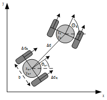
Odometry involves the use of data from motion sensors to estimate changes in an agent's position over time. A human analogy is the counting of steps to guess how far you've walked. For robots or machines, these "steps" can come from sensors such as wheel rotations or inertial sensors. Although odometry provides continuous updates, it is prone to accumulation of errors, also known as "drift."
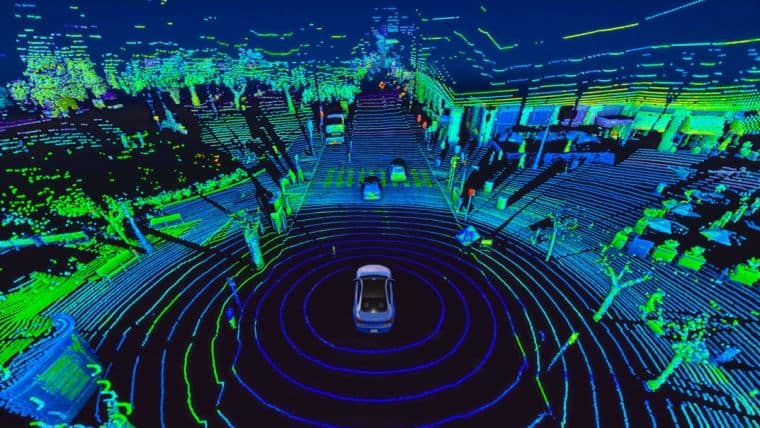
Point clouds are sets of data points in space or 3D coordinates, usually produced by ranging sensors such as 3D LiDAR scanners or stereo cameras. Typically, these sensors emit various forms of electromagnetic radiation and measure the reflected signals to calculate the distance of objects from the scanner, thus generating a "point cloud" that represents the environment. Point clouds are essential in SLAM as they provide the raw data for the map of the environment that the SLAM system is trying to create.
There are typically 2 ways to obtain point cloud data[3]:
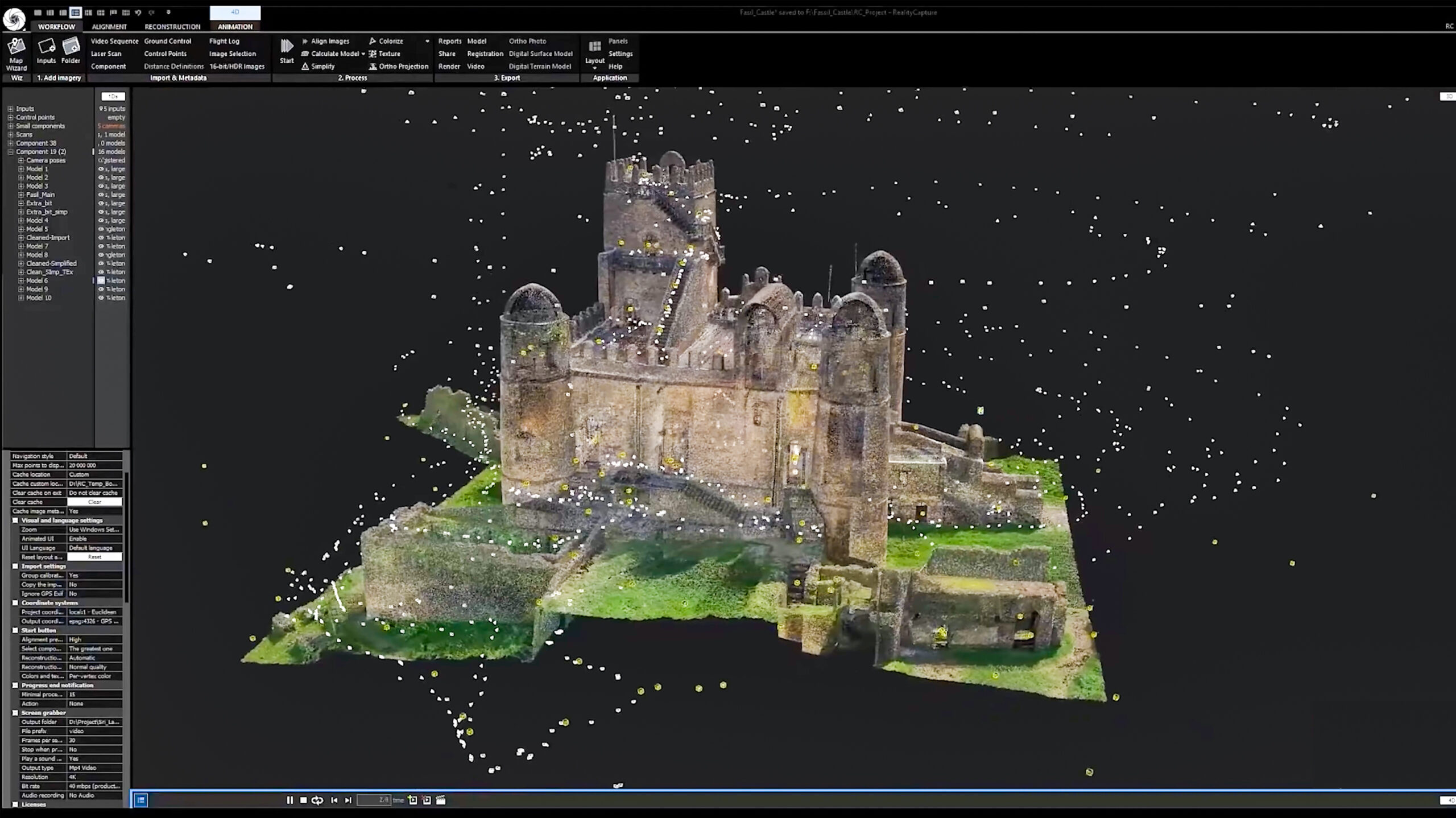
As its name suggests, this method involves using image-based sensors (e.g. RGB cameras, stereo cameras, or compound eye cameras) and computer vision techniques (e.g. stereo photography or photogrammetry) to extract 3D information from the 2D images obtained by the sensors. While there may be higher computational costs and more dependence on good lighting conditions for reliability, the sensors themselves are typically much cheaper than LiDAR sensors. In addition, using cameras would also capture the color and lighting information about the environment, which would otherwise be lost when using LiDAR SLAM.

LiDAR, which stands for "Light Detection and Ranging" involves shooting out numerous laser rays onto the surrounding surfaces and recording the time taken for each ray to return to the sensor. While LiDARs come at a higher monetary cost, it is usually more precise than camera sensors as they can capture fine details and are less susceptible to visual ambiguities. It is usually more robust as well, working in dark or foggy conditions that challenge vSLAM.
In this section, we will go through scenarios with increasing complexity and incrementally develop the SLAM algorithm to accommodate the challenges introduced in each scenario.
Ref: Understanding SLAM Using Pose Graph Optimization | Autonomous Navigation, Part 3[4]


We start off by approaching this problem naively by considering the behaviors in an ideal world. We will be able to solve the localization part of the problem simply through the odometry data from the robot (left image). At the same time, there will also be no uncertainty or errors in the lidar measurements, which gives the robot perfect information about its surroundings, solving the mapping part of the problem too.

As the robot drives around the environment, it continues picking up more lidar points about its surroundings and also keeps track of its relative position using its odometry data while doing so.

Now consider our less ideal situation where the lidar is accurate but the odometry sensor isn't as accurate (e.g. wheel slippage is a common source of error for wheel encoders). When the robot moves around in the real world, the computer estimates the point cloud points relative to the odometry, causing mismatch between the ground truth point cloud and the recorded point cloud.

The crux of SLAM algorithms lies in the pose graph optimization solution. In pose graph nomenclature, a "pose" refers to the positional data from the lidar and the odometry at a point in time, and an "edge" refers to the constraints between poses. By optimizing the constraints, we can align the point cloud data between poses to obtain the best approximation possible of the entire environment.

Finally, to identify and correct previously visited areas, we can "close the loop" and reduce cumulative errors in the map and location estimates. This step is crucial for maintaining accurate mapping over time by reconciling the robot's current understanding of its location with past observations.
While the core intuition described in Section 3 is highly simplified, the actual implementations of SLAM often involve an advanced understanding of robotics, mathematics, and computer science. Nevertheless, to provide a holistic technical appreciation of SLAM, we will take a closer look at 3 of the most popular algorithms that serve as the backbone for SLAM systems. These algorithms are what translate sensor data into information used in the robots' decision-making process and for building coherent maps. Understanding these algorithms, even at a high level, therefore allows us to have a better appreciation for the sophistication and challenges involved in SLAM technology.
| Extended Kalman Filters (EKF) | Particle Filters (Monte Carlo Localization) | Graph-Based SLAM |
|---|---|---|
| EKF is one of the pioneering algorithms in SLAM. It addresses the inherent non-linearity of robot navigation by approximating the state and measurement updates. Think of EKF as a navigator who not only corrects the route based on the latest observations but also predicts future positions by smoothing out the erratic nature of sensor data. | With Particle Filters, the SLAM system adopts a probabilistic approach (think of it as placing bets on where the robot might be). Each particle represents a guess, and as the robot moves and gathers more sensor data, these guesses are refined, converging on the robot's likely position. | This algorithm involves drawing a map as a network of landmarks and paths (think nodes and edges). Graph-Based SLAM solves the SLAM problem by finding the most probable arrangement of these network nodes that aligns with sensor observations; it is essentially solving a giant, dynamic puzzle. |

SLAM's versatility enables its application across diverse sectors:
- Consumer Robotics: Household robots, like autonomous vacuum cleaners, use SLAM to navigate around homes efficiently and avoiding obstacles and entire areas are covered.
- Industrial Automation: In warehouses, SLAM allows robots to find and retrieve items, keeping track of both the items' locations and their own.
- Autonomous Vehicles: Self-driving cars use SLAM for navigating roads and adjusting to new environments in real-time.
- Aerospace: Drones and planetary rovers use SLAM to navigate and map terrains in GPS-denied environments such as Mars or the moon's surface.
- Underwater Exploration: Autonomous underwater vehicles use SLAM to explore the ocean's depths where radio signals cannot reach and remote control of the vehicles is impossible.
From our discussion on SLAM thus far, it is evident that it is a computationally intensive process. While the technicalities of the machine learning implementation within SLAM were not covered in detail, it is worth noting that SLAM often involves many hours of tuning and optimization of the hyperparameters when exploring different environments. For example, an exploration of the unpredictable terrains of a rainforest can be significantly more challenging than an exploration of a more structured setting like an apartment complex - consequently, the algorithm has to be turned to take the noisy environment into account.
Thus, recent research in SLAM primarily focuses on optimizing these algorithms for efficiency and accuracy. As recently as last year, UCLA's very own VECTOR lab (Verifiable and Control-Theoretic Robotics Laboratory) made a notable advancement in improving localization accuracy and mapping clarity, while simultaneously reducing the computational load. According to their test flights, the team discovered that their drone, embedded with their new algorithm, performed 20% faster and 12% more accurately than those armed with current state-of-the-art algorithms[5].
In conclusion, SLAM empowers machines to understand and move through the world, attaining new information or capabilities that were previously impossible to achieve without autonomous navigation. Its versatility also extends across countless sectors and has played crucial roles in the advancement of many technologies. As autonomous navigation engineers and enthusiasts, it is meaningful to not only appreciate the complex mathematical challenge that SLAM is but also appreciate how this technology enabled the evolution of modern automation and robotics.
[1] H. Durrant-Whyte and T. Bailey, "Simultaneous localization and mapping: part I," in IEEE Robotics & Automation Magazine, vol. 13, no. 2, pp. 99-110, June 2006, doi: 10.1109/MRA.2006.1638022.
[2] https://www.mathworks.com/discovery/slam.html
[3] https://www.baeldung.com/cs/slam
[4] https://www.youtube.com/watch?v=saVZtgPyyJQ
[5] https://samueli.ucla.edu/ucla-engineers-unveil-algorithm-for-robotic-sensing-and-movement/