Delta Parallel Robot - Trajectory Planning

---

A word from me: This repository is dedicated to studying the different trajectory planning methods (theory + practical). Newer Version of This Repository is Available at link

for the complete report on the theory of delta parallel robot please refer to my internship report this will be a step by step demonstration of how I experimented the different methods of trajectory planning for a Delta Parallel robot End-Effector

Overview:

• Inverse and Forward Kinematics
• Motion Planning (Point-To-Point)
  • 3-4-5 Polynomial interpolation
  • 4-5-6-7 Polynomial interpolation
  • Trapeoidal
• Motion Planning (Multi-Point)
  • cubic-spline
  • Trapezoidal
  • Jacobian (incomplete)

INVERSE AND FORWARD KINEAMTICS

with trajectory planning there are two fundemental questions we need an answer for:

1. given a specific location in the real world, what values should my robot's joint be set to in order to get the End-Effector there? (inverse kinematics)
2. given the setting of my joints, where is my EE in real world coordinates? (forward kinematics)

Theory

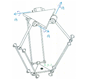
The Delta robot is a 3-DOF robot that consists of two parallel platforms. One of them, which we call the EE platform, is capable of moving and the other one, which we call base platform, is not capable of that. These two platforms are connected with three arms. Each arm has one pin and two universal joints (as shown in the figure) that connect two solid rods. The rod which is connected to base platform by the pin, is called the active rod, and the other one is called the passive rod. The center of the base and EE platforms are marked as $O$ and $O'$ respectively. The pin is denoted as A, the universal joint connecting the passive and active rods, is denoted as B. The universal joint connecting the EE platform and the passive rod is denoted as C.

$\overrightarrow{(O O')} + \overrightarrow{(O' C_i)} = \overrightarrow{(O A_i)} + \overrightarrow{(A_i B_i)} + \overrightarrow{(B_i C_i)}$ (Equation 1)

• IK: so you'll need to solve this equation and find $\theta_{ij}$ with respect to the other variables. this will solve the inverse kinematics problem. $\theta_{1j}$ are the angles of the actuator joints.
• FK: for forward kinematics it, the equation number 1 is solved for $p_x, p_y, p_z$ (position of the EE) with respect to other variables (which is a much easier problem that IK)

References

• here's a good playlist for learning FK and IK

• Delta Robot Inverse Kinematics

• Delta Robot Inverse Kinematics method 1

• Delta Robot Inverse Kinematics method 2

Python implementation

you can see my python implementation of IK:

• method 1
• method 2

MOTION PLANNING POINT-TO-POINT MOVEMENT

this section is dedicated to answer how should you go about writing a code for point to point movement (moving the EE from point 1 to point 2 in 3d space )

3-4-5 Polynomial Interpolation

In order to represent each joint motion, a fifth-order polynomial $s(\tau)$ is used here. meaning that, if $\theta_0$ and $\theta_1$ and the corresponding time instants of $t_0$ and $t_1$ are given, the path between them can be interpolated by use of a fifth order polynomial that outputs a predicted $\theta_{pred}(t)$ that $t \ \in \ [t_0, \ t_1]$

Theory

the polynomial is shown in the following form $$s(\tau) = a\tau^5 + b\tau^4 + c\tau^3 + d\tau^2 + e\tau + f$$ such that $$0 \leq s \leq 1 \quad 0 \leq \tau \leq 1$$ and $$\tau = \frac{t}{T}$$ we will thus aim at a normal polynomial that, upon scaling both its argument and the polynomial itself, will allow us to represent each of the joint variables $\theta_j$ throughout its range of motion so that: $$\theta(t) = \theta_I + (\theta_F - \theta_I)s(\tau)$$ and $\frac{d \theta}{dt}, \ \frac{d^2 \theta}{d t^2}, \ \frac{d^3 \theta}{d t^3}$ are calculated by defferentiating the above formula with the boundary conditions at $$s(0), \ s^\prime (0), \ s^{\prime \prime} (0), \ s(1), \ s^\prime (1), \ s^{\prime \prime} (0)$$

python implementation

• POINT TO POINT MOVEMENT (3-4-5 polynomial): moveing from point to point in the direction desired --> trajectory_planning_345.py

4-5-6-7 Polynomial Interpolation

The problem with 3-4-5 polynomial is that the jerk at the boundary can't be set to zero, for this problem we use a higher degree of polynomial, namely, 7-th deg polynomial.

Theory

with the steps similar to the last section and the added boundary conditions of $s^{\prime \prime \prime}(0), \ s^{\prime \prime \prime}(1)$ we solve the system of question generated from the boudary conditions.

python implementation

• POINT TO POINT MOVEMENT (4-5-6-7 polynomial): we repeat what we've done for sub-step 2 but with a 7th order polynomial --> trajectory_planning_4567.py

Source

3-4-5 polynomial and 4-5-6-7 polynomial point to point movement, you can learn about this in the book "Fundamentals of Robotic Mechanical Systems, theory, methods, and Algorithms, Fourth Edition by Jorge Angeles - chapter 6"

Trapezoidal point to point movement

In Trapezoidal method we have 3 phases,

• Phase 1: constant positive acceleration
• Phase 2: constant velocity
• Phase 3: constant negetive acceleration

$V = a.t \quad for \quad 0 \leq t \leq T_a$
$V = V_{max} \quad for \quad T_a \leq t \leq T - T_a$
$V = -a.t \quad for \quad T-T_a \leq t \leq T$

Pytohn implementation

you can find the codes related to trapezoidal point to poitn movement in this source code

This is the resultant plot:

S-Curve

as a concept, s-curve is the better version of trapezoidal. strictly speaking, it has seven phases instead of three. as explained blow in mathemathis terms:

$a = J.t \quad for \quad T_0 \leq t \leq T_1$
$a = a_{max} \quad for \quad T_1 \leq t \leq T_2$
$a = J(T_3 - t) \quad for \quad T_2 \leq t \leq T_3$
$a = 0 \quad for \quad T_3 \leq t \leq T_4$
$a = -J(t - T_4) \quad for \quad T_4 \leq t \leq T_5$
$a = -a_{max} \quad for \quad T_5 \leq t \leq T_6$
$a = -J(T_7 - t) \quad for \quad T_6 \leq t \leq T_7$

MOTION PLANNING MULTI-POINT MOVEMENT

this section is dedicated to planning out a specific trajectory for the robot to go through

Cubic-spline

one way of interpolating a path of $n+1$ points in space, is by a polynomial of degree $n$. This way might work for 3 or 4 points, but fir higer degree polynomials it can be very computationally expensive. Another way which is much better in terms of computational power needed, is using $n$ polynomials of degree $p$ that $p << n$. The overall function $s(t)$ defined in this manner is called a spline of degree $p$.

python implementation

• CIRCLE MOVEMENT: cubic spline with assigned initial and final velocities --> trajectory_planing_cubic_spline.py

Computation of the coefficient for assigned initial and final velocities plot:

• CIRCLE MOVEMENT: cubic spline with assigned initial and final velocities and acceleration --> trajectory_planing_cubic_spline_4.4.4.py

Computation of the coefficient for assigned initial and final velocities and acceleration plot:

source

cubic spline (book Trajectory Planning for Automatix Machines and Robots by Luigi Biagiotti and Claudio Melchiorri)

1. cubic spline with assigned initial and final velocities (part 4.4.1)
2. cubic spline with assigned intial and final velocities and acceleration (part 4.4.4)
3. smoothing cubic spline (part 4.4.5)

Trapezoidal - multi-points

a very common method to obtain trajectoryies with a continuous velocity profile is to use linear motions with parabolic blends, characterized therefore by the typical trapezoidal velocity profiles.

To achieve something like this first we need to initiate a form of velocity prfile and then modify it

Python Implementation

If the method from point to point trapezoidal movement is used directly for multi-point, velocity becomes zero quite often and in every pre-defined point in the path, which is not acceptable. this kind of behaviour can be seen in the plot below:

\textbf{Theory and algorithm of modifying the velocity profile above}

after modifying this velocity profile we get the following plots:

Jacobian

The jacobian matrix relates velocity of EE to the velocity of actuator joints with the relation: $\vec{v} = J \dot{\vec{\theta}}$

theory

for the IK we have the equations as followed

• $p_x \cos(\Phi_i) - p_y \sin(\Phi_i) = R - r + a \cos(\theta_{1i}) + b \sin(\theta_{3i}) \cos(\theta_{2i} + \theta_{1i})$ (equation 1)
• $p_x \sin(\Phi_i) + p_y \cos(\Phi_i) = b \cos(\theta_{3i})$ (equation 2)
• $p_z = a \sin(\theta_{2i}) + b \sin(\theta_{3i}) \sin(\theta_{2i} + \theta_{1i})$ (equation 3)

from these equation we solve for $\theta_{ij}$ (solution of IK) and solve for $p_x, p_y, p_z$ (solution of FK)

further explanation in the following pdf that i've written according the mentioned references: jacobian, IK and FK

1. what is Jacobian matrix and how it is calculated
2. how jacobian matrix is used in delta robot trajectory palanning
3. detailed calculation and analysis of Jacobian matrix in delta robot

python implementation

• jacobian file: IK, FK, jacobian matrix calculation