Data Structure

RECAP

• Linked List ( Linkedlist -> head, Node -> value, next pointer )
  • Singly
    • Each node contain a pointer that point to the next node.
    • The pointer of the last node of the linkedlist point to NULL.
  • Doubly
    • Each node contains a pointer that point to the previous node and the next node.
    • The previous pointer of the head node of the linkedlist point to NULL.
  • Circular
    • The next pointer of the last node point to the head node of the linkedlist.
• Stacks ( Stack -> top and Node -> value, next pointer (point from top to down))
  • Each node contains a pointer and value.
  • The next pointer of the base node (the bottom of the stack) point to NULL.
• Queue ( Queue -> front and rear, Node -> value, next (point to the node behind) )
  • The next pointer of the last queue point to null.
• Trees
• Heaps
• Graphs
• Hash Tables

---

• A data structure is a model where data is organized, managed and stored in a format that enables efficient access and modification of data.
• Different forms of data may require different types of data structures.
• A program built using improper data structures will be therefore inefficient or unnecessarily complex. It is neccessary to have a good knowledge of data structures and understand where to use the best one.

Inbuilt Data Structure

Inbuild data structurs are provided by most programming languages. They may used to derive other data structures.

• Arrays -> Stores elements of the same type in a contiguous block of memory, can accessed by a common identifier.
• Structures -> Creates a data type that can be used to group items of different types into a single type.

Abstract Data Type (ADT)

Abstract Data Types are defined by its behaviour from the point of view of the user of the data.

It defines it in terms of:

• Possible values
• Operations on data
• The behaviour of these operations.

The difinition of ADT only mentions what operations are to be performed but not how these operations will be implemented. It does not specify how the data is being handled under the hood, this is known as abstraction.

Example of ADT:

• Linked Lists: Consists of nodes, where each node points to some other node forming a sequence.
• Stacks: The insdrtion and deletion operations are performed at only one end. It follows the LIFO principle.
• Queues: The insertion and deletion operations are performed at two different ends. It follows the FIFO principle.
• Trees: Hierarchical data structure where the information is represented in the form of a parent and children.
• Heaps: Specialized tree-based data structure that satisfies the heap property.
• Graphs: Consists of nodes and edges used to represent relations between pairs of objects.
• Hash Tables: Data is stored in an associative manner. A hash function is used to map the data to array positions.

---

Linked List

• Operations - Inserting at the Beginning, Inserting at the End, Inserting at a specific position - Deleting at the Beginning, Deleting at the End, Deleting at a specific position - Show List, Get value at position, Get size

Advantage over an array

• Not Fixed in Size
• Efficient Insertion and Deletion: Insertion and deletion are efficient and take constant time as only the links are manipulated, not the actual memory location of the actual elements.

Disadvantage over an array

• Slightly more memory usage
• Sequential Access
• Difficult revers traversal: Difficulties arise in liked lists when it comes to revers traversing in a singly linked list. This can be resolved using doubly linked list, but this again increase memory as we have to store the previous reference pointer.

Uses of a Linked List

• Implementation other data structure: It is used to implement other data structures such as stacks, queues and non-linear ones like trees and graphs.
• Hash Chaining: It has used in hash chaining for the implementation in open chaining.

Types of Linked List

1. Singly Linked List
   • A singly linked list is the simplest type of linked list in which every node contains some data and a pointer to the next node.
   • Allows traversal of data only in one way.
2. Doubly Linked List
   • Every node has two pointers: next and previous. This allows for reverse traversal anywhere in the list.
3. Circular Linked List
   • Last node connect to the first node, forming a loop.
   • The last node contain a pointer to the first node of the list.
   • While traversing a circular linked list, we can begin at any node and traverse the list in any direction, forward or backward, until we reach the same node where we started.

---

Stack

A stack is a linear data structure which stores its elements in particular order. This order followed by a stack is known as LIFO (Last in First Out).

An example of real life phenomena of stacks is of plates stacked over one another on a table. The plate which is at the top is the first one to be removed, it is not possible to remove the last plate unless the above plates have been removed, following the principle Last In First Out.

Examples in Programming

1. UNDO functionality in text editors: are based on a stack. Every change in the document is added to stack and upon an UNDO request, the last change is referred by popping it from the stack.
2. Parentheses checker: the ordered manner of the stack could be used for checking the proper closing of parentheses. Every opening parentheses is pushed on to the stack and for every correct closing parentheses, it is poped off. Irregularities can then be detected if they mismatch.
3. Expression parsing: using stacks can help evaluate expressions faster using postfix or prefix notation.

Properties

1. Follows LIFO (Last In First Out Order), the last element that is inserted is pushed out first.
2. A pointer keeps track of the stack's topmost (or last) element. This is manipulated on the basis of operations to be performed to know keep track of most recent element.

Stack Manipulation Operations

1. Push Operation: When an element is inserted into the stack, it is said that the element is pushed into the stack. The top pointer is moved up to point to the element that is inserted.
2. Pop Operation: When an element is removed from the stack, it is said that the element is popped from the stack. The top pointer is moved down to point to the element below the removed element.
3. Peek Operation: Peek is an operation that returns the value of the topmost element of the stack without deleting it from the stack.

---

Queues

Queue is a linear data structure which unlike the stack is open at both ends. If follows the FIFO (First In First Out) principle, which means that the element that is inserted first is removed first.

Real Life Examples of Queus

1. An example of a queue is the queue we see everyday in our lives. People join a queue from the end and get out of the queue from the front, following the FIFO principle.
2. A queue is used in process scheduling in the Operating System. A series of precesses wait in a queue waiting to be executed when required resources are free.

Properties

1. Follows the FIFO (First In First Out Order), the first element that is inserted, is removed first.
2. Two pointers keep track of the front and rear ot the queue, whenever insertion or deletion takes place, these two pointers are updated accordingly to track the last and first element.
3. Insertion takes place from the rear and deletion from the front.

Types of Queues

Queues and their functions can be modified to have some additional advantages, some of the other types of queues are:

1. Double Ended Queus (Deque) A deque is a list in which the elements can be inserted or deleted at either end. These are further of two types:
   1. Input Restricted Queue: Where insertion takes place only from the rear end, deletion can take place from both ends.
   2. Output Restricted Queue: Where deletion takes place from only the front, however insertion can take place from both ends.
2. Priority Queues Priority queue is like a regular queue or stack data structure, but where additionally each element has a 'priority' associated with it. In a priority queue, an element with high priority is served before an element with low priority.

This can be helped in operations where priority is important for executing operations in a certain order.

3. Circular Queue (Circular Buffer) Additional resources: https://www.geeksforgeeks.org/circular-queue-set-1-introduction-array-implementation/

A circular queue is a queue that uses a single, fixed-size buffer as if it were connected end-to-end.

Circular queue is a good implementation for a queue that has fixed maximum size, as their is no shifting involved and the whole queue can be used up for storing all the elements, which is not possible in an array implementation of linear queue.

Circular Queue is a linear data structure in which the operations are preformed based on FIFO (First In First Out) principle and the last position is connected back to the first position to make a circle. It is also called 'Ring Buffer'.

In a normal Queue, we can insert elements until queue becomes full. But once queue becomes full, we can not insert the next element even if there is a space in front of queue.

---

Trees

Additional Resources

• https://www.gatevidyalay.com/tree-data-structure-tree-terminology/
• https://www.geeksforgeeks.org/extended-binary-tree/

A tree is widely used data structure that simulates a hierarchical tree structure, with a root value and the subtrees as children, represented as a set of linked nodes. The children of each node could be accessed by traversing the tree until te specific value is reached.

Advantages of trees

1. Trees (with some ordering e.b., BST) provide moderate access/search (quicker than a Linked List).
2. Trees provide moderate insertion/deletion (quicker that Arrays) speed.

Uses in programming

1. File System structure: directories and subdirectories of a file system can be efficiently be represented by trees.
2. DOM structure: HTML pages are rendered using a DOM structure which contains all the tags used in the page under a tree-like structure.
3. Router algorithms: use trees to figure out a path for the data to follow efficiently.

Terminology used in trees

• Root: The first node in a tree is called as Root Node. Every tree must have one Root Node.
• Parent Node: The node which is a predecessor of any node is called as Parent Node, that is, the node which has a branch from it to any other node is called as the Parent node.
• Child Node: The node which is descendant of any node is called as Child Node. Any parent node can have any number of child nodes. All the nodes except root are child nodes.
• Sibling: Nodes which belong to the same Parent are called as Siblings.
• Leaf Node: In a tree data structure, the node which does not have a child is called a Leaf Node. They are also known as External Nodes or Terminal Nodes.
• Internal Nodes
  • The node which has at least one child is called an Internal Node.
  • Internal nodes are also called as non-terminal nodes.
  • Every non-leaf node is an internal node.
• External Nodes: The node which has no child is called an External Node.
• Degree
  • Degree of a node is the total number of children of that node.
  • Degree of a tree is the highest degree of a node among all the nodes in the tree.
• Level
  • In a tree, each step from top to bottom is called as level of a tree.
  • The level count starts with 0 and increments by 1 at each level or step.
• Height
  • Total number of edges that lies on the longest path from any leaf node to a particular node is called as height of that node.
  • Height of a tree is the height of root node.
  • Height of all leaf nodes = 0.
• Depth
  • Total number of edges from root node to a particular node is called as depth of that node.
  • Depth of a tree is the total number of edges from root node to a leaf node in the longest path.
  • Depth of the root node = 0.
  • The terms "level" and "depth" are used interchaneably.
• Path: The sequence of Nodes and Edges from one node to another node is called as PATH between that two Nodes.
• Subtree
  • In a tree, each child from a node forms a subtree recursively.
  • Every child node forms a subtree on its parent node.
• Forest
  • A forest is a set of disjoint trees.

Types of trees

1. Binary Trees
   • In a normal tree, every node can have any number of children. A Binary tree is a special type of tree in which every node can have a maximum of 2 children. One is known as left child and the other as right child.
   • Binary Tree Representation
     • Array Representation: The binary tree is represented in a 1-Dimensional array.
     • Linked List Representation: A doubly linked list is used to represent a binary tree. Here, every node consists of 3 fields. First field for storing left child's address, second for storing data and third for storing right child's address.
   • Types of Binary Trees
     1. Strictly Binary Tree: A binary tree in which every node has either two or zero children is a Strictly Binary Tree.
     2. Complete Binary Tree: A binary tree in which every internal node has exactly two children and all leaf nodes are at same level is a Complete Binary Tree.
     3. Extended Binary Tree
        • The full binary tree obtained by adding dummy nodes to a binary tree is called as Extended Binary Tree.
        • Extended binary tree is a type of binary tree in which all the null sub tree of the original tree are replaced with special nodes called external nodes whereas other nodes are called internal nodes.
     4. Threaded Binary Tree
        • Threaded Binary Tree is also binary tree in which all left child pointers that are NULL points to its in-order predecessor, and all right child pointers that are NULL points to its in-order successor.
        • Inorder traversal of a Binary tree can either be done using recursion or with the use of a auxiliary stack. The idea of threaded binary trees is to make inorder traversal faster and do it without stack and without recursion. A binary tree is made threaded by making all right child pointers that would normally be NULL point to the inorder successor of the node (if it exists).
        • There are two types of threaded binary trees.
          1. Single Threaded: Where a NULL right pointers is made to point to the inorder successor (if successor exists)
          2. Double Threaded: Where both left and right NULL pointers are made to point to inorder predecessor and inorder successor respectively. The predecessor threads are useful for reverse inorder traversal and postorder traversal.
        • The threads are also useful for fast accessing ancestors of a node.
2. Binary Search Trees
   • Terminologies:
     • Inorder successor
     • Inorder predecessor
   • Additional Resources:
     • https://www.geeksforgeeks.org/binary-search-tree-set-2-delete/
   • A Binary Search Tree is a binary tree that additionally satisfies the binary search property.
   • Binary Tree Property
     • This property state that the key in each node must be greater than or equal to any key stored in the left sub-tree, and less than or equal to any key stored in the right sub-tree.
   • Operations in Binary Search Tree
     • Searching
     • Insertion
     • Deletion
3. Multiway Search Trees
   • A multiway tree can have more than one value per node. They are written as m-way trees where the m means the order of the tree. A multiway tree can have m-1 values per node and m children (m ways). Although, not every node needs to have m-1 values or m children.
4. AVL Trees
   • An AVL tree is a self-balancing binary search tree. A binary tree is said to be balanced, if the difference between the heights of left and right subtrees of every node in the tree is either -1, 0, or +1. This is known as the Balance Factor.
   • Balance Factor
     • Balance Factor = height(left_subtree) - height(right_subtree)
   • Rebalancing
     • During a modifying operation (e.g. insert, delete), if the height difference of more than 1 arises between two subtrees, the parent subtree has to be 'rebalanced' to satisfy the AVL property.
     • These are done by tree rotations, which moves the keys in such a manner that there order is preserved, but the balance factor is also satisfied.
   • AVL Tree Rotations
     • Rotation is the process of moving the nodes to either left or right to make tree balanced. There are 4 types of rotations:
       1. Single Left Rotation (LL Rotation)
       2. Single Right Rotation (RR Rotation)
       3. Left Right Rotation (LR Rotation)
       4. Right Left Rotation (RL Rotation)

Binary Tree Traversals

A binary tree is traversed when one needs to access or display its elements. Each method produces a different order of elements that may be useful in scenarios when needed.

• Traversal Methods
  1. Inorder [Left - Root - Right]
     • In this traversal, the left child node is visited first, then the root node is visited and later we go for visiting right child node.
  2. Preorder [Root - Left - Right]
     • In this traversal, the root node is visited first, then its left child and later its right child.
  3. Postorder [Left - Right - Root]
     • In this traversal, left child node is visited first, then its right child and then its root node.

---

Heaps

A heap is a specialized tree-based data structure that satisfies the heap property. It can be of 2 types: max heap and min heap.

The Heap Property

The heap property says that is the value of Parent is either greater than or equal to (in a max heap) or less than or equal to (in a min heap) the value of the Child.

Uses in programming

1. Heapsort: One of the best in-place sorting methods with no quadratic worst-case scenarios. This is because the minimum or maximum element is always the root of the tree.
2. Implementing prioriy queus: the highest (or lowest) priority element is always stored at the root.
3. Selection algorithms: A heap allow access to the the min or max element in constant time, and other selections (such as median or kth-element) can be done in sub-linear time on data that is in heap.
4. Graph algorithms: By using heaps as internal traversal data structures, run times can be reduced by polynomial order.

Heap Operations

• Finding Maximum/Minimum
  • Finding the node which has maximum or minimum value is easy. Due to the heap property, it will be always the root node, hence we can access it in constant time.
• Insertion
  • The new heap would not necessarily satisfy the heap property, we have to make it satisfy the heap property
    • Step 1: Insert the node like in a normal tree.
    • Step 2: If the new Node is greater/lesser than its parent, swap it with it's parent.
• Deletion
  • An element is always deleted from the root of the heap. So, deleting an element from the heap is done in the following steps:
    • Step 1: Replace the root node's value with the last node's value.
    • Step 2: Delete the last node.
    • Step 3: Sind down the new root node's value so that the heap again satisfies the heap property.

---

Graph

A graph is a non-linear data structure consisting of nodes and edges. The nodes are sometimes also reffered to as vertices and the edges are lines or arcs that connect any two nodes in the graph. More formally a Graph can be defined as,

A Graph consists of a finite set of vertices (or nodes) and set of Edges which connect a pair of nodes.

Properties of graphs

1. A graphs G is defined as an ordered set (V, E), where V(G) represents the set of vertices and E(G) represents the edges that connect these vertices.
2. A graph can be directed or undirected:
   • In an undirected graph, edges do not have any direction associated with them.
   • In a directed graph, edges from an ordered pair. If there is an edge from A to B, then there is a path from A to B but not from B to A.

Uses in programming

Graphs are used to solve many real-life problems. Graphs are used to represent networks. The networks may include paths in a city or telephone network or circuit network. Graphs are also used in social networks like linkedIn, Facebook. For example, in Facebook, each person is represented with a vertex (or node). Each node is a structure and contains information like person id, name, gender, locale etc.

Terminology used in Graphs

• Vertex: A individual data element of a graph is called as Vertex.
• Edge: An edge is a connecting link between two vertices. An Edge is also known as Arc.
• Undirected Graph: A graph with onl undirected edge is said to be undirect graph.
• Directed Grpah: A graph with only directed edges is said to be directed graph.
• Mixed Graph: A graph with undirected and directed edges is said to be mixed graph.
• Origin: If an edge is directed, its first endpoint is said to be origin of it.
• Destination: If an edge is directed, its first endpoint is said to be origin of it and the other endpoint is said to be the destination of the edge.
• Adjacency: Two node or vertices are adjacent if they are connected to each other through an edge.
• Path: Path represents a sequence of edges between the two vertices.
• Degree: Total number of edges connected to a vertex is said to be degree of that vertex.
• In-Degree: Indegree of a vertex is the number of edges which are coming into the vertex.
• Out-Degree: Outdegree of vertex is the nubmer of edges which are going out from the vertex.
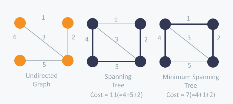
• Minimum Spanning Tree (MST): A minimum spanning tree (MST) is a subset of the edges of a connected, edge-weighted (un)directed graph that connects all the vertices together, without any cycles and with the mimimum possible total edge weight.
• Simple Graph: A graph is said to be simple if there are no paralled and self-loop edges.
• Directed acyclic graph (DAG): A directed acyclic graph (DAG) is a graph that is directed and without cycles connecting the other edges. This means that it is impossible to traverse the entire graph starting at one edge.
• Weighted Graph: A weighted graph is a graph in which a number (known as the weight) is assigned to each edge. Such weights might represent for example costs, legths or capacities, depending on the problem.
• Complete Graph: A complete graph is a graph in which each pair of vertices is joined by an edge. A complete graph contains all possible edges.
• Connected Graph: A connected graph is an undirected graph in which every unordered pair of vertices in the graph is connected. Otherwise, it is called a disconnected graph.

Representation of Graphs

A graph can be represented in memory in 2 ways: 1. Adjacency Matrix 2. Adjacency List

Graph Traversals

Graph traversal is technique used for searching a vertex in a graph. It is also used to decide the order of vertices to be visit in the search process. A traversal algorithms is careful not to get into loops and repeatedly visit the same nodes.

There are 2 common graph traversal algorithms:

1. Breadth First Search: Explores all of the neighbor nodes at the present depth prior to moving on to the nodes at the next depth level.
   • Breadth-first search (BFS) is a graph search algorithm that begins at the root node and explores all the neighboring nodes. Then for each of those nearest nodes, the algorithm explores their unexplored neighbor nodes, and so on, until it finds the specified node.
   • A queue is used as an auxiliary data structure to keep track of the neighbouring nodes.
   • Properties:
     1. Time complexity: In the worst case, breadth-first search has to traverse through all paths to all possible nodes. Therefor, the time complexity can be expressed as O(|E| + |V|) which is the sum of all vertices(V) and edges(E).
     2. Space Complexity: In the breadth-first search algorithm, all the nodes at a particular level must be saved until their child nodes in the next level have been visited. The space complexity is therefore proportional to the number of nodes at the deepest level of the graph.
     3. Completeness: Breadth-first search is said to be a complete algorithm because if there is a solution, breadth-first search will find it regardless of the kind of graph. But in case of an infinite graph where there is no possible solution, it will diverge.
2. Depth First Search: Explores as far as possible along each branch before backtracking.

Other Algorithms

• Togological Sorting: Linear ordering of vertices such that for every directed edge uv from vertex u to vertext v, u comes before v in the ordering.

---

Hash Tables

A Hash table is a data structure in which keys are mapped to array positions by a hash function.

A value stored in a hash table can then be searched in O(1) time, by using the same hash function which generates an address from the key. The process of mapping the keys to appropriate locations (or indices) in a hash table is called hashing.

Advantages of Hashing

The main advantage of hash tables over other data structure is speed. The access time of an element is on average O(1), therefore lookup could be performed very fast. Hash tables are particulary effiecient when the maximum number of entries can be predicted in advance.

Hash Functions

A hash function is a mathematical formula which, when applied to a key, produces an value which can be used as an index for the key in the hash table. The main aim of a hash function is that elements should be uniformly distributed.

Properties of a Good Hash Function

• Uniformity: A good hash function must map the keys as evenly as possible. This means that the probability of generating every hash value in the output range should roughly be the same. This also helps reducing collisions.
• Deterministic: A hash procedure must be deterministic - meaning that for a given input value, the function must always generate the same hash value.
• Low Cost: The cost of executing a hash function must be small, so that using the hashing technique becomes preferable over other traditional approaches.

Uses in Programming

1. Identification Database: A hash function can make a unique signature from never changing data like our Date of Birth. This can be used in combination of other variables to uniquely identify a person.
2. Search Engines: As the number of pages to be crawled is huge, a hash function is used to determine if the page is unique or it had already been crawled before, without comparing the whole webpage.

Different Hash Functions

• Division Method: It is the most simple method of hashing an integer x. This method divides x by M and then uses the remainder obtained. Generally, it is best to choose M to be a prime number because making M a prime number increases the likelihood that the keys are mapped with a uniformity in the output range of values.
• Multiplication Method
• Mid-Square Method

Bucket Hashing

Additional Resources: https://opendsa-server.cs.vt.edu/OpenDSA/Books/CS3/html/BucketHash.html

One implementation for closed hashing groups hash table slots into buckets. The M slots of the hash table are divided into B buckets, with each bucket consisting of M/B slots.

The hash function then assigns each record to the first slot within one of the buckets. If the slot is already occupied, then the bucket slots are searched sequentially until an open slot is found.

If a buckey is entirely full, then the record is stored in an overflow bucket of infinite capacity at the end of the table. All buckets share the same overflow bucket.

An efficient implementation will use a hash function that distributes the record evenly among the buckets so that as few records as possible go into the overflow bucket.

Collisions

Collisions occur when the hash function maps two different keys to the same location. As two records cannot be stored in the same location.

The method used to solve the problem of collisions is called the collision resolution technique.

There are two popular collision resolution techniques:

1. Open Addressing: Once a collision takes place, open addressing or closed hasing computes new position using a probe sequence and the next record is stored in that position.
   • There are some well known probe sequences:
     1. Linear Probing: in which the interval between probes is fixed, often 1 is used.
     2. Quadratic Probing: in which the interval between probes increase quadratically.
     3. Double Hashing: in which the interval between probes is fixed for each record but is computed by another hash function.
2. Seperate Chaining: In chaining, each location in a hash table stores a pointer to a linked list that contains all the key values that were hashed to that location. As new collisions occur, the linked list grows to accommodate those collisions forming a chain. Searching for value in a chained hash table is as simple as scanning a linked list for an entry with the given key. Insertion operaion appends the key to the end of the linked list pointed by the hashed location. Deleting a key requires searching the list and removing the element.

---