Overview and Comparison of Features
This article gives an overview over all feature point algorithms implemented in PCL. The following criteria are important when describing an algorithm:
- Category: Local, regional, global
- Does it extend other known methods (e.g. Name is based on Spin Images)
- Does it require a specific input format?
- High level overview so that a beginner / technical interested person understands the purpose and methodology of the algorithm(s).
- Process chain in 3 to 5 points
- Use cases
See Feature overview
| Feature Name | Supports Texture / Color | Local / Global / Regional | Best Use Case |
|---|---|---|---|
| PFH | No | L | |
| FPFH | No | L | 2.5D Scans (Pseudo single position range images) |
| VFH | No | G | Object detection with basic pose estimation |
| CVFH | No | R | Object detection with basic pose estimation, detection of partial objects |
| RIFT | Yes | L | Real world 3D-Scans with no mirror effects. RIFT is vulnerable against flipping. |
| RSD | No | L | |
| NARF | No | L | 2.5D (Range Images) |
| ESF | No | G |
- Local
The PFH extends the previous work on Surflet-Pair-Relation Histograms (Wahl et. al.).
- Surflet-pair-relation histograms: a statistical 3D-shape representation for rapid classification
- A point cloud consisting of a set of oriented points P. Oriented means that all points have a normal n.
- This feature does not make use of color information.
- Iterate over points in the point cloud P.
- For every point Pi (i is the iteration index) in the input cloud all neighbouring points within a sphere around Pi with the radius r are collected. This set is called Pik (k for k neighbours)
- The loop regards pairs of two points in Pik, say p1 and p2. The point whose normal has the smaller angle to the vector p1-p2 is the source point ps, the other one is the target point pt.
- Four features are calculated which together express the mean curvature at the target point pt. Those are combined and put into the equivalent histogram bin. For further details on the feature calculation see the original paper: http://www.willowgarage.com/papers/learning-informative-point-classes-acquisition-object-model-maps

- Create normals for all points in P
- Estimate features for a point Pi in P: The set of k-neighbours in the radius r around the point Pi (Pik) is taken. Four features are calculated between two points. The corresponding bin is incremented by 1. A point feature histogram (PFH) is generated.
- The resulting set of histograms can be compared to those of other point clouds in order to find correspondences.
- Local
The FPFH extends the Point Feature Histogram (PFH).
- A point cloud consisting of a set of oriented points P. Oriented means that all points have a normal n.
- This feature does not make use of color information.
As the FPFH is derived from the PFH it works a lot alike. But there are some optimisation steps making FPFH faster.
- Iterate over points in the point cloud P.
- For every point Pi (i is the iteration index) in the input cloud all neighbouring points within a sphere around Pi with the radius r are collected. This set is called Pik (k for k neighbours)
- The loop only regards pairs of point Pi with each of its neighbours (remember in PFH the loop would generate pairs of Pi and its neighbours and also between _Pi_s neighbours!). In such a pair the point whose normal has the smaller angle to the vector p1-p2 is the source point ps, the other one is the target point pt.
- Three features (four in PFH, the distance between Ps and Pt was left out) are calculated which together express the mean curvature at the target point pt. Those are combined and put into the equivalent histogram bin.
- As in FPFH only direct pairs between the query point Pi and its neighbours are taken into consideration (far less computation) the resulting histogram is called SPFH (Simple Point Feature Histogram).
- The last step is new: To recompensate the "lost" connections the neighbours' SPFHs are added to Pi's SPFH according to their spatial distance. For further details on the feature calculation see the original paper: http://files.rbrusu.com/publications/Rusu09ICRA.pdf

- Create normals for all points in P
- Estimate features for a point Pi in P: The set of k-neighbours in the radius r around the point Pi ( Pik ) is taken. Three features are calculated between two points (only between Pi and its neighbours!). The corresponding bin is incremented by 1. A simple point feature histogram (SPFH) is generated.
- To reach more points and connections (up to 2 times r) the SPFH of the neighbours are added weighted according to their spatial distance as a last step.
- The resulting set of histograms can be compared to those of other point clouds in order to find correspondences.
- Global
The VFH extends the Fast Point Feature Histogram (FPFH).
- A point cloud consisting of a set of oriented points P. Oriented means that all points have a normal n.
- This feature does not make use of color information.
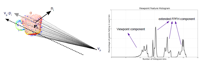
- Calculate the centroid pc of the point cloud and its normal nc. Calculate the vector between the viewpoint and the centroid vc and normalize it.
- The VFH consists of two components: A viewpoint component and an extended FPFH component.
- To map the viewpoint component iterate over all points in P and calculate the angle between their normal and vc. Increment the corresponding histogram bin.
- For the viewpoint component simply calculate the FPFH at the centroid pc setting the entire surrounding point cloud P as neighbours.
- Add the two histograms together.
- For further details on the feature calculation see the original paper: http://www.willowgarage.com/sites/default/files/Rusu10IROS.pdf
- Estimate the centroid and its normal in the point cloud. Calculate the normalized vector vc between the viewpoint and the viewpoint.
- For all points calculate the angle between their normal and vc.
- Estimate the FPFH signature for the centroid with all remaining points set as neighbours.
- Regional
The CVFH extends the Viewpoint Point Feature Histogram (VFH).
- A point cloud consisting of a set of oriented points P. Oriented means that all points have a normal n.
- This feature does not make use of color information.
- The result of computing the point and normal centroid for the entire cloud can be entirely different once points are missing due to occlusion and sensor limitations. That's why VFH descriptors turn out entirely different once essential points are missing from a cloud.
- CVFH creates stable regions (clusters). From the point cloud P a new cluster Ci is started from a random point Pr that hasn't been assigned to any cluster yet. Every point Pi in P is assigned to that cluster if there exists a point Pj in Ci so that their normals are similiar and they are in a direct neighbourhood (compare angle and distance thresholds). Clusters with too few points are rejected.
- Compute the VFH on each cluster.
- Add a shape distribution quotient to each histogram that expresses how the points are distributed around the centroid.
- For further details on the feature calculation see the original paper: http://ieeexplore.ieee.org/xpl/articleDetails.jsp?arnumber=6130296

- Subdivide the point cloud into clusters (stable regions) of neighbouring points with similiar normals.
- Calculate the VFH for each cluster.
- Add the shape distribution component (SDC) to each histogram.
- Local
The RIFT feature extends SIFT (Lowe).
- Object recognition from local scale-invariant features (http://ieeexplore.ieee.org/xpls/abs_all.jsp?arnumber=790410&tag=1)
- A point cloud consisting of a set of textured points P. Without textures this feature will not produce any usable results.
- Intensity Gradients: http://docs.pointclouds.org/trunk/classpcl_1_1_intensity_gradient_estimation.html
- Iterate over points in the point cloud P.
- For every point Pi (i is the iteration index) in the input cloud all neighbouring points within a sphere around Pi with the radius r are collected. This set is called Pik (k for k neighbours)
- An imaginary circle with n segments (the projection of the sphere perpendicular to the normal of Pi) is fitted to the surface. Here n corresponds to the number of distance bins in the implementation.
- All neighbours of Pi are assigned to a histogram bin according to their distance d < n and gradient angle position theta < g (g denotes the number of gradient bins in the implementation). Theta is the angle between the gradient direction and the vector pointing outwards the circle from the center.
- For further details on the feature calculation see the original paper: http://hal.inria.fr/docs/00/54/85/30/PDF/lana_pami_final.pdf

- For each point Pi in P sample all k neighbours around Pi.
- Assign all neighbours to a histogram according to their distance d and their gradient angle theta.
- The resulting set of histograms can be compared to those of other point clouds in order to find correspondences.
- Local
The NARF feature extends a few concepts of SIFT (Lowe).
- Object recognition from local scale-invariant features (http://ieeexplore.ieee.org/xpls/abs_all.jsp?arnumber=790410&tag=1)
- A range image RI of a scene.
- NARF is not only a descriptor but also a detector. You might want to run the interest point detector over the data set first: http://docs.pointclouds.org/trunk/classpcl_1_1_narf_keypoint.html
- Iterate over all interest points in the range image RI.
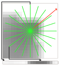
- For each point Pi create a small image patch by looking at it along its normal. The normal is the Z-axis of the image patch's local coordinate system where Pi is at (0,0). The Y-axis is the world coordinate system Y-Axis. The X-axis aligns accordingly. All neighbours within the radius r around Pi are transfered into this local coordinate system.
- A star pattern with n beams is projected on the image patch. For each beam a score in [-0.5,0.5] is calculated. Beams have a high score if there are lots of intensity changes in the cells lying under the beam. This is calculated by comparing each cell with the next adjacent one. Additionally cells closer to the center contribute to the score with a higher weight (2 in the middle, 1 at the edge).
- Finally the dominant orientation of the patch is calculated to make it invariant against rotations around the normal.
- For further details on the feature calculation see the original paper: https://www.willowgarage.com/sites/default/files/icra2011_3dfeatures.pdf
- For each keypoint Pi in RI sample all neighbours around Pi and transform them into a local coordinate system with Pi being at O
- Project a star pattern on the image patch and count the intensity changes under each beam to get the beam's score. In the calculation beams closer to the center have more weight. The scores are normalized to [-0.5,0.5].
- Iterate over all beams and find the dominant orientation of the image patch.
- Local
- --
- A point cloud consisting of a set of oriented points P. Oriented means that all points have a normal n.
- This feature does not make use of color information.
- Iterate over points in the point cloud P.
- For every point Pi (i is the iteration index) in the input cloud all neighbouring points within a sphere around Pi with the radius r are collected. This set is called Pik (k for k neighbours)
- For each neighbour Pikj in Pik the distance between Pi and Pikj and the angle between their normals is calculated. These values are assigned to a histogram that characterizes the curvature at the point Pi.
- Using these values an imaginary circle with an approximated radius rc can be fitted through the two points (see image). Note that the radius becomes infinite when the two points are located on a plane.
- As the query point Pi can be part of multiple circles with its neighbours only the minimum and the maximum radius are kept and assigned to Pi as output. The algorithm accepts a maximum radius paramteter above which points will be considered as planar.

- For each point Pi in P sample all k neighbours around Pi.
- Assign all neighbours to a histogram according to their distance d and their undirected normal's angle.
- Assume that pairs of Pi with each of its neighbours describe a circle (see image). Find the minimum and maximum radius of all the spheres Pi describes with its neigbours.
- The resulting set of histograms and the radii can be compared to those of other point clouds in order to find correspondences.
- Local
- A3, D2, D3 shape description functions: Matching 3D Models with Shape Distributions (Osada et. al.)
- D2 improvements (IN, OUT, MIXED): Using Shape Distributions to Compare Solid Models (Ip et. al.)
- A point cloud consisting of a set of points P.
- This feature does not make use of color information.
- Start a loop that will sample 20,000 points from the point cloud P.
- Every iteration samples three random points Pri, Prj, Prk.
- D2: For the D2 function calculate the distance between Pri and Prj. Then check if the line connecting the two points lies entirely on the surface (IN), outside the surface (OUT) or both (MIXED). Increment one of D2's subhistograms (either IN, OUT or MIXED) at the previously calculated distance bin. As three points were sampled, two other distances can be calculated in this iteration.
- D2 ratio: There is another histogram that captures the ratio between parts of each line lying on the surface and in free space.
- D3: For the D3 function calculate the square root of the area of the triangle between Pri, Prj and Prk. This is done equivalent to D2 as the area is also classified into IN, OUT and MIXED. Increment the corresponding histogram bins of the D3 histogram.
- A3: For the A3 function calculate the angle between the three points. Again this function is classified into IN, OUT and MIXED. This time the line opposite to the angle is used. Increment the corresponding A3 histogram bin.
- At the end of the loop we end up with a global descriptor containing 10 subhistograms (64 bins each): D2 (IN, OUT, MIXED, ratio), D3 (IN, OUT, MIXED), A3 (IN, OUT, MIXED).
- Read the entire paper for more information: http://ieeexplore.ieee.org/xpl/articleDetails.jsp?arnumber=6181760

- Start a loop that randomly samples 20,000 points from the point cloud P. Each round sample three points Pri, Prj, Prk.
- For pairs of two points calculate the distance between each other and check if the line between the two lies on the surface, outside or intersects the object (IN, OUT or MIXED). Increment the bin corresponding to the calculated distance in one of D2's three subhistograms.
- For the previous line find the ratio between parts of that line lying on the surface or outside. The result should be 0 for entirely outside, 1 for entirely on the surface and all values from MIXED lines are distributed in between. Increment the corresponding bin of the D2 ratio histogram.
- For triplets of points build a triangle and calculate the angle between two sides and classify the side of the angle's opposite of the triangle (IN, OUT, MIXED). Increment the corresponding angle bin in either the IN, OUT or MIXED subhistogram of A3.
- For the previous triangle calculate the square root of the area and classify the area into IN, OUT or MIXED. Increment the corresponding area bin in either the IN, OUT or MIXED subhistogram of D3.