Home
BIPAC has been published in IEEE EMBC 2015 [1] and the paper was awarded as the open finalist of student paper competition. It is a seed-based imaging method to estimate the phase-amplitude coupling (PAC) between seed activity and the activity of other regions. The program of BIPAC from has been written as a plug-in of the Matlab Software Brainstorm. Please download the program of BIPAC from Github: https://github.com/Hui-Ling/BeamformerSourceImaging. The .m files should be placed in the following folder: $HOME\.brainstorm\process.
Please contact me to get the access of example data (Email: hlchan@cs.nctu.edu.tw). After obtaining access right, the example data can be downloaded here: Tutorial_FingerLifting.zip.
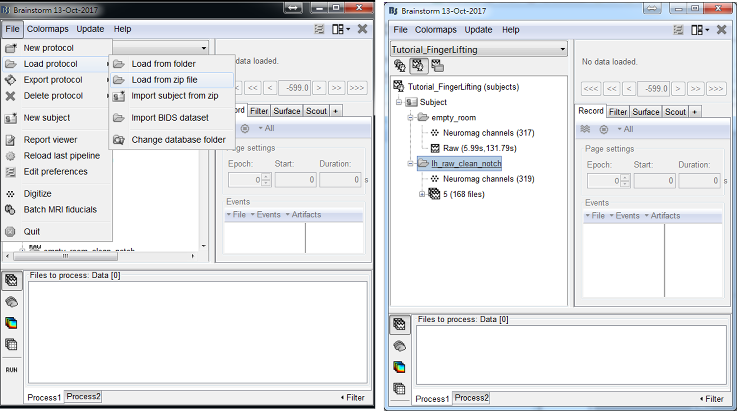
The MEG data used in this tutorial was acquired by Elekta Neuromag Vector View 306 Channel MEG during a self-paced finger lifting experiment, which has been used to demonstrate the accuracy of maximum contrast beamformer (MCB) [2]. An empty-room MEG data is also included, which has been processed by using Apply SSP & CTF compensation in Brainstorm. The anatomy data used in this tutorial is the MRI template Colin27, which is built in Brainstorm. To load the example data into Brainstorm, select File > Load from zip file and then select Tutorial_FingerLifting.zip. A subject containing empty-room data and finger-lifting data will be shown in the data explorer window.
- Step1: Drag trials of preprocessed MEG trials to input window, and press RUN
- Step2: Select Frequency > Power spectrum density (Welch) > Edit (PSD options). Set Output to be save average PSD values (across trials), which can largely reduce the data size of output results. Then press OK and press Run.

- Step3: Double click on the output file PSD: 1/1000ms Avg, Power (MEG GRAD) to show power spectrum density. Then right-click on the figure and select 2D Sensor cap.

- Step4: Use left or right arrow on keyboard to show the power distributed on the 2D sensor cap for a different frequency. Find the frequency bands that you are interested in for further cross-frequency analysis.

-
Step1: Drag trials of preprocessed MEG trials to input window, and press RUN.
-
Step2: Select Frequency > Time-Frequency (Morlet wavelets) and then set spectral flattening to be 1/f compensation. Then edit Morlet wavelet options by setting Output to save average time-frequency maps (across trials), which largely reduces the data size of output results. Then press OK and press Run.

- Step 3: Right-click on the output file and select 2D Layout (maps) from the popup window. Then the time-frequency maps of all GRAD channels will be displayed. You may left-click and move-down or -up to change the colormap.

- Step 4: Left-click on any of the time-frequency map to individually display the map in a new window. Find the frequency bands that you are interested in for further cross-frequency analysis.

The above results demonstrate that high gamma activity in the sensorimotor area may couple to the alpha and beta activity in the same area or other areas. This tutorial describes the procedure to compute the spatiotemporal distribution of cross-frequency coupling between the gamma activity at a sensorimotor seed and the whole brain activity in the alpha/beta frequency bands by using BIPAC. Hereafter, you will see the operations including (1) selection of a seed location based on the peak location of gamma brain activity, (2) extraction of the seed activity, and (3) estimation of seed-based alpha-gamma and beta-gamma PAC maps.
The following steps demonstrate how to obtain seed location by using MCB. MCB is used to estimate the significance of sources in the manner of power contrast between active state and control state. In this tutorial, the control state is from the data recorded in an empty room.
-
Step 1: Drag the empty-room file Raw (5.99s,131.79s) to Process1 and press RUN.
-
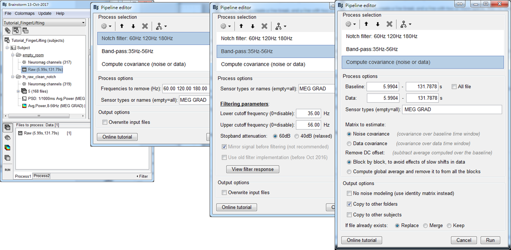
Step 2: In the pipeline editor, select Pre-Process > Notch filter, which is to reduce power-line contamination (60 Hz in Taiwan). Then select Pre-Process > Bandpass filter, which is to filter out signal at gamma band (35-56 Hz). Finally, select Source > Compute Covariance (noise or data) as well as check Noise covariance and Copy to other folders. Press Run.
-
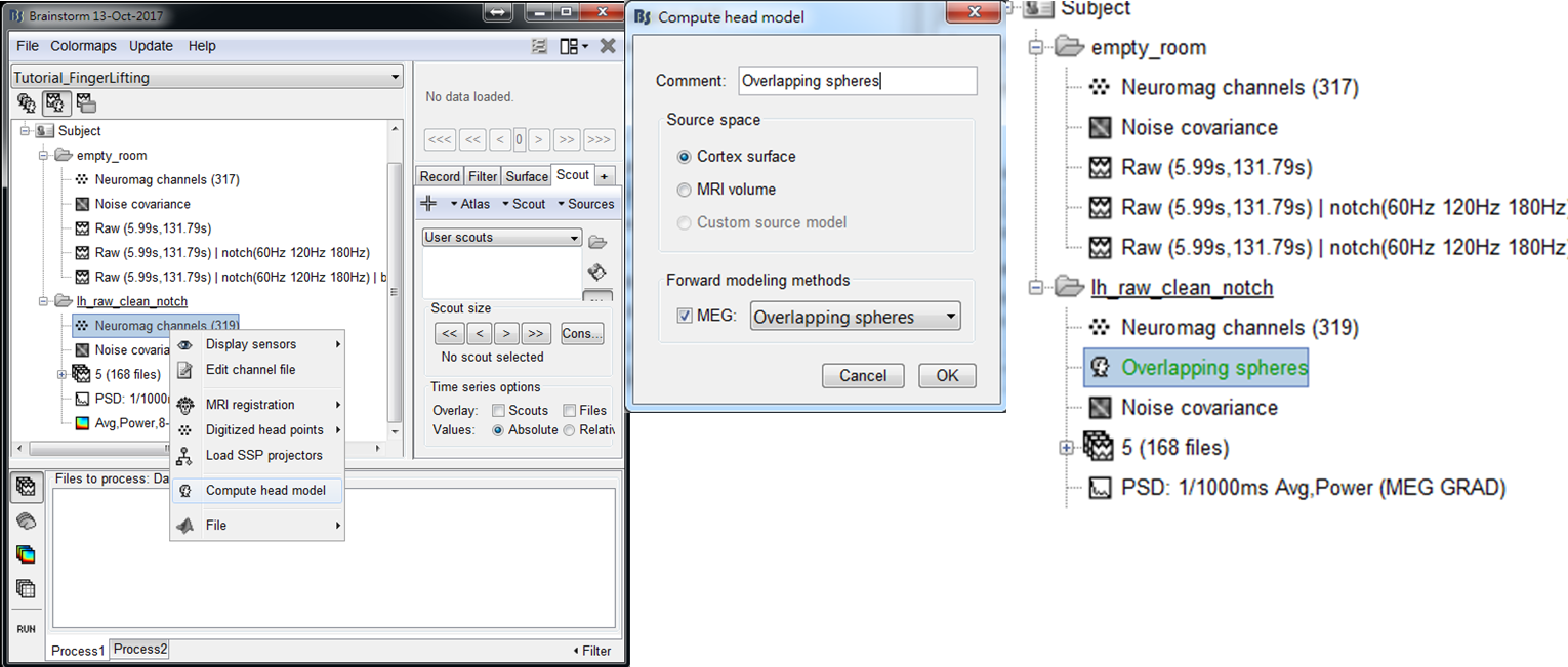
Step 1: Right-click on the channel file of lh_raw_clean_notch: Neuromag channels (319). Select Compute head model of the popup window.
-
Step 2: Select Cortex surface and press Run. Then Overlapping spheres will be displayed in the data explorer window. The green color indicates the current selection of the head model for the use in source estimation.
-
Step 3: Drag trials of preprocessed MEG trials to Process1, and press RUN.
-
Step 4: Select Pre-process > Bandpass to filter out the data at gamma frequency band (35-56 Hz). Then select Source > Beamformer: Maximum Contrast (speedup). After setting the parameters, press Run. The meaning of every parameter is described below:
- Options: Dipole orientation - Select unconstrained and set the time range to be [-500, 500] ms.
- Options: Spatial filter - Check Save spatial filters because it is required for the extraction of seed activity. Set time range to be [-500, 500] ms. Increasing regularization parameter may obtain a smoother cortical distribution.
- Options: Active state (for f-statistic map) - DOI indicates the time period for the computation of f maps. The size of a sliding window represents the length of the active state. In this tutorial, the setting represents that a 35-ms sliding window slides within [-600, 600] ms in a step of 4 ms.

- Step 5: Drag the output f maps gamma source: MCB/fmap (Unconstr, no bl, ws:-581-579ms, tr:4ms) to Process1. Select Average > Average time and set the time window to average f maps ([-500, 500] ms in this tutorial). Press Run.

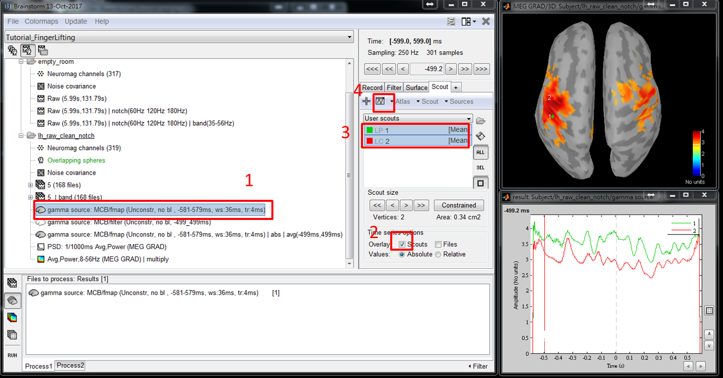
- Step 6: Double clicked on the output file gamma source: MCB/fmap (Unconstr, no bl, ws:-581-579ms, tr:4ms)|abs|avg(-499ms, 499ms) to display the averaged f map. Press 0, 1, 2, ..., or 9 to show a different view of results.

There are two ways to select seed: data-driven selection or manual selection.
- Data-driven selection: Select the peak position as a new scout by using Scout > Sources > maximal value (new scout).
- Manual selection: Left-click on the cross mark and then left click on the location you want to select as seed.

The temporal dynamics of activity at scouts may provide more information for you to select a seed. To show the temporal dynamic, double click on the file gamma source: MCB/fmap (Unconstr, no bl, ws:-581-579ms, tr:4ms), check Scouts to overlay, select all of the scouts that you are interested in, and click the waveform mark.
In this step, the gamma activity at the selected seed location of every trial is extracted and then concatenated to be a unique matrix. The matrix will be used as a reference signal for BIPAC computation.
-
Step 1: Put trials of bandpass MEG data, 5 | band (168 files), to Process1. Select the brain mark. Then press RUN.
-
Step 2: Select Extract > Scouts time series. Select one of the scouts as the seed (scout 1 in this tutorial). Check Concatenate output in one unique matrix. Then press Run.

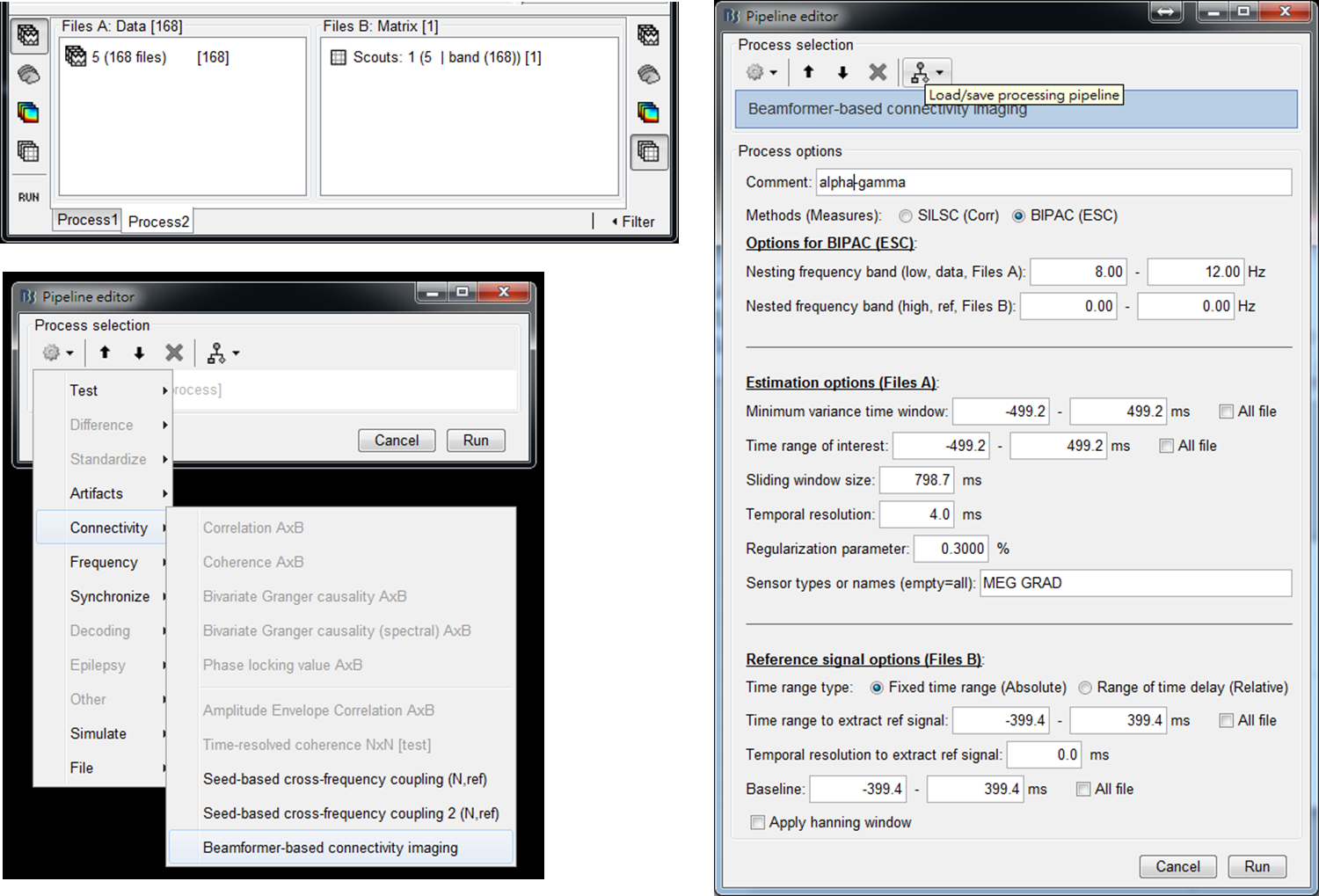
The computation of BIPAC requires two types of input files: (1) trials of MEG measurements and (2) a matrix containing all trials of seed activity. Instead of Process1, running BIPAC requires selecting Process2 as input windows. Hereafter, we will show the steps to obtain alpha-gamma and beta-gamma PAC maps referenced at the selected seed location (Scout 1).
Step 1: Put trials of MEG data to FilesA of Process2 and the file of seed activity, Scouts: 1(5 | band (168)), to FilesB of Process2. Press RUN.
Step 2: Select Connectivity > Beamformer-based connectivity imaging.
Step 3: Set parameters for the computation of alpha-gamma PAC and then press Run.
- Comment - The prefix of the name of output files.
- Methods (Measures) - SILSC is for seed-based correlation imaging [3] and BIPAC is for seed-based PAC imaging. In this tutorial, BIPAC is selected.
- Options for BIPAC (ESC) - Nesting and nested frequency bands for PAC estimation, which should be set as alpha ([8,12]Hz) and gamma ([35,56]Hz) bands for the computation of alpha-gamma PAC. The ranges of a frequency band can be set as [0,0]Hz if the inputs are bandpass signals. In this tutorial, the reference signals placed in FileB are trials of seed activity in gamma band. Thus, the nested frequency band can be set as [0,0]Hz.
- Estimation options (Files A) - Minimum variance time window is used in the computation of beamforming spatial filter. It should cover the time ranges that brain sources are activated. Time range of interest is to define the time period to compute PAC and a sliding window moves within this time period in a step of Temporal resolution. For every step, a PAC map is computed. A small value of temporal resolution increases computation time. The Minimum variance time window should be large enough to cover Time range of interest. Previously, the time-frequency maps show strong alpha and beta oscillations before performing finger-lifting and some of the oscillations decrease before or after performing the tasks. Thus, we set a large time window [-500, 500]ms for Minimum variance time window and Time range of interest to cover these changes of oscillations. Sliding window size defines the size of the sliding window and should be the same as the length of the reference signal, which is 800 ms in this tutorial. Regularization parameter influences the shape of a spatial filter, where a large value prevents overfitting but also allows more leakages from nearby sources. The default value 0.3% is selected based on our simulation experiments.
- Reference signal options (Files B) - Select Fixed time range (Absolute) and set Time range to extract ref signal as [-400, 400]ms. In this case, the gamma activity at seed during [-400,400]ms is used to compute the coupling with the alpha activity of other regions during [-500,300]ms, [-496,304]ms, ..., [-300, 500]ms. Set Temporal resolution to extract ref signal as 0 ms. This parameter is for the use in the study of multiple reference signals (function under development) [3]. Baseline defines the time period of baseline and a setting of [0,0] ms represents no baseline correction for the reference signal.

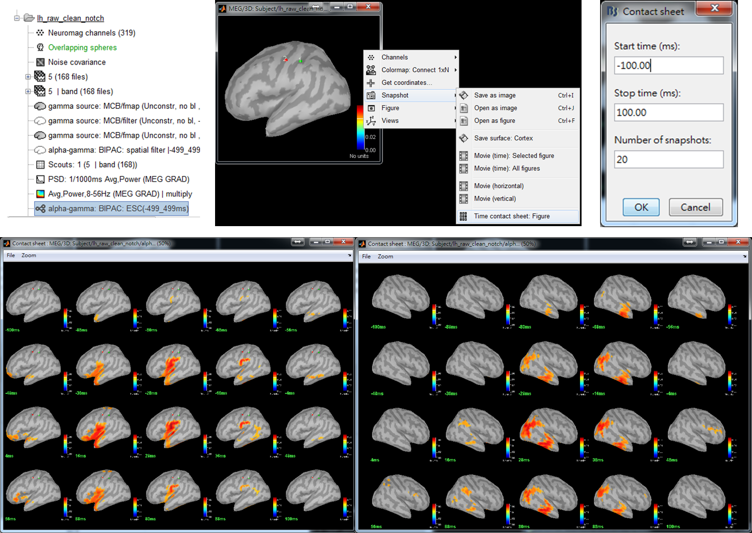
Step 4: Double-click on the output file alpha-gamma: BIPAC: ESC(-499_499ms) to show PAC maps. Right-click on the popup window and select Snapshot > Time contact sheet: Figure. In the window of Contact sheet, set Start time as -100 ms, Stop time as 100 ms, and Number of snapshots to be 20. Press OK.
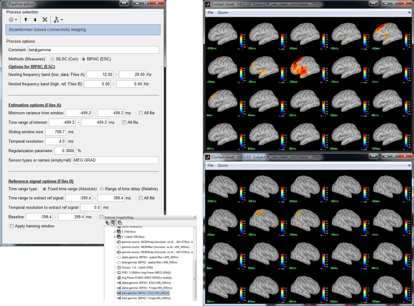
Step 5: Set parameters for the computation of beta-gamma PAC and then press Run. Except for [12,28]Hz of Nesting frequency band, the parameter values are the same as those used in Step 3.
[1] Chan, H.-L., Y.-S. Chen, L.-F. Chen, and S. Baillet (2015), 'Beamformer-based imaging of phase-amplitude coupling using electromagnetic brain activity', 37th Conf. Proc. IEEE Eng. Med. Biol. Soc. (Milan, Italy).
[2] Chen, Y.-S., C.-Y. Cheng, J.-C. Hsieh, and L.-F. Chen (2006), 'Maximum contrast beamformer for electromagnetic mapping of brain activity', IEEE Trans. Biomed., 53 (9), 1765-74.
[3] Chan, H.-L., L.-F. Chen, I.-T Chen, Y.-S. Chen (2015), 'Beamformer-based spatiotemporal imaging of linearly-related source components using electromagnetic neural signals', NeuroImage, 114, 1-17.
[4] Chan, H.-L., Y.-S. Chen, L.-F. Chen (2011), 'Maximum multiple-correlation beamformer for estimating source connectivities in electromagnetic brain activities', 33rd Conf. Proc. IEEE Eng. Med. Biol. Soc. (Boston, USA).