2021_Characterization of genomes using k mer spectra analysis_SAGA
Before we start
# log to the cluster
# ssh <your_name>@saga.sigma2.no

# Go to your directory
cd $USERWORK

# copy all the kmer histograms
cp -r /cluster/projects/nn9458k/oh_know/teachers/kamil/data/data_for_genomescope .

# start interactive job we will use to fit several models
srun --ntasks=1 --mem-per-cpu=5G --time=02:00:00 --qos=devel --account=nn9458k --pty bash -i

# activate conda environment with genomescope (it will probably drop some warnings / errors, but should at the end load the conda env anyway)
module --force purge
module load Miniconda3/4.9.2
conda init bash
conda config --add channels defaults
conda config --add channels conda-forge
conda config --add channels bioconda
source ~/.bashrc

conda activate /cluster/projects/nn9458k/oh_know/.conda/kmer_tools
Now that we are on the cluster with activated env, we can finally fir all the genomescope models. If you are not sure how to fit a model, see the crayfish example bellow. If you managed to get everything done yesterday, you can either explore your own data, or there are a bunch of pretty messed up k-mer spectra of nematodes in the nematode direcotry.
- Begonia
- Bombina
- Cape Bees
- Crayfish
- Mercurialis
- Springtails
- Stick insects
- Strawberry
- BONUS Nematodes
Procambarus virginalis., the marbled crayfish is an asexual triploid with a supererepetitive genome. This is the reason why if fit the model to truncated k-mer spectrum, the estimated genome size is more than 1GB below the expected genome size. The monoploid size is known to be somewhere between 3 - 3.5 Gbp.
mkdir -p 01_crayfish

# naive fit of the turnicated data
genomescope.R -i data_for_genomescope/crayfish/P_virginalis_trimmed_turnicated_SRR5115143,SRR5115144,SRR5115145,SRR5115146,SRR5115147,SRR5115148_k17.hist -p 3 -k 17 -o 01_crayfish/ -n P_virginalis_trimmed_turnicated
# very high heteoryzogosity and VERY small genomes size, it is very likely that 1n peak has a low lower coverage

# let's set a prior on the coverage to one third of previous fit 16x (quite often the real 1ns are 1/2 for diploid / tetraploid species and 1/3 for triploid species)
genomescope.R -i data_for_genomescope/crayfish/P_virginalis_trimmed_turnicated_SRR5115143,SRR5115144,SRR5115145,SRR5115146,SRR5115147,SRR5115148_k17.hist -p 3 -k 17 -l 17 -o 01_crayfish/ -n P_virginalis_trimmed_turnicated_l20
# the genome size is still just 2.2G, which is a LOT less than what we would expect, let's see how counting all the kmers will help

# this the same model, but fit to a histogram that contains 200000 more rows with high all the supererepetitive kmers (coverage >10000x)
genomescope.R -i data_for_genomescope/crayfish/P_virginalis_trimmed_SRR5115143,SRR5115144,SRR5115145,SRR5115146,SRR5115147,SRR5115148_k17.hist -p 3 -k 17 -l 18 -o 01_crayfish/ -n P_virginalis_trimmed

# for comparison, you can also check, how much trimming the reads helped to clarify the kmer spectra by fitting the model to the raw kmer spectra
genomescope.R -i data_for_genomescope/crayfish/P_virginalis_raw_SRR5115143,SRR5115144,SRR5115145,SRR5115146,SRR5115147,SRR5115148_k17.hist -p 3 -k 17 -l 18 -o 01_crayfish/ -n P_virginalis_raw
Finally, we also provede a histogram of the diploid sister species P. fallax. This sequencing library is unfortunately with very low coverage and therefore the model does not converge on the right monoploid coverage without setting a prior. One truly hidden developer's trick for genomes with poor coverage is to add parameter --num_rounds=1 which somehow makes GenomeScope mimic GenomeScope v1, which works better on these low-coverge genomes. Check this twitter thread.
genomescope.R -i data_for_genomescope/crayfish/P_fallax_SRR5115152_k17_full.hist -p 2 -k 17 -o 01_crayfish/ -n P_fallax --num_rounds=1
# the model says the haploid size is 1.75Gbp, which is about half what we expected, let's also fit a model with smaller prior on coverage

genomescope.R -i data_for_genomescope/crayfish/P_fallax_SRR5115152_k17_full.hist -p 2 -k 17 -l 15 -o 01_crayfish/ -n P_fallax_l15 --num_rounds=1
# this is more like it
Now, get all the models to your computer and check the plots. It has been suggested the clonal marbled crayfish turned asexual due to autopolyploidization. Do you think it's plausible/parsimonious given the values of heterozygosities you see?
KAT for genome assembly QC
For this bit we will be using the tse-tse genome assemby and reads in /cluster/projects/nn9458k/oh_know/teachers/kamil/data/tse-tse/
KAT is pre-installed on saga, so to load it we only have to type module add KAT/2.4.2-foss-2019a-Python-3.7.2. To make sure it has worked, now you can just call KAT by typing kat or kat comp, which is the tool we will be using within KAT.
The whole command is something like this:
kat comp -t <n of threads> -o <output directory, e.g. tse-tse_reads_vs_assembly> <input1-readfile> <input2-genomeassembly>
You could run it in an inteactive node, by typing first srun --ntasks=12 --mem-per-cpu=12G --time=02:00:00 --qos=devel --account=nn9458k --pty bash -i
And then running it like this (using, for example, one of the read files):
kat comp -t 8 -o tse-tse_reads_vs_assembly \
/cluster/projects/nn9458k/oh_know/teachers/kamil/data/tse-tse/Glossina_14_R1.fastq.gz \
/cluster/projects/nn9458k/oh_know/teachers/kamil/data/tse-tse/ncbi-genomes-2021-09-12/GCF_014805625.1_Yale_Gfus_2_genomic.fna.gz
This may take a while (~30', or you could ask for more resources when running srun) and because we wanted to make it a quick job, we also only selected one of the smallest read files (Glossina_14_R1.fastq.gz), and therefore the coverage of the histograms is not very high. But now you know how to run in on your/other datasets!
To run it on a script with both your R1 and R2 reads, you can use something like:
#!/bin/bash

#SBATCH --job-name=KATcomp
#SBATCH --account=NN9458K
#SBATCH --time=00-04:00:00
#SBATCH --cpus-per-task=8
#SBATCH --mem-per-cpu=12G

#to call the read files
R1=$1
R2=$2
# to call the assembly file
FILE_WITH_ASSEMBLY=$3
# the prefix for the output
OUTPUT_PREFIX=$4

#setting up our environment
module purge
module add KAT/2.4.2-foss-2019a-Python-3.7.2

#running KAT comp
kat comp -t 8 -o "$OUTPUT_PREFIX" \
"$R1 $R2" "$FILE_WITH_ASSEMBLY"

exit
We have a copy of this script in /cluster/projects/nn9458k/oh_know/teachers/kamil/data/kat_two_read_files.sh, so you can copy that one into your home directory :)
And then submit the job with:
sbatch kat_two_read_files.sh /cluster/projects/nn9458k/oh_know/teachers/kamil/data/tse-tse/Glossina_12_R1.fastq.gz \
/cluster/projects/nn9458k/oh_know/teachers/kamil/data/tse-tse/Glossina_12_R2.fastq.gz \
/cluster/projects/nn9458k/oh_know/teachers/kamil/data/tse-tse/ncbi-genomes-2021-09-12/GCF_014805625.1_Yale_Gfus_2_genomic.fna.gz \
tse-tse-ref_vs_reads
explanation
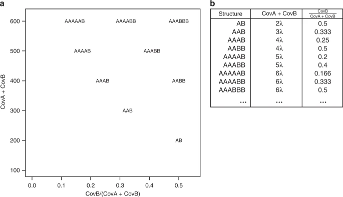
Sometimes, k-mer spectra is hard to read, figuring out which peak is which can be difficult. That is the reason why we developed smudgeplot - a tool that searches for all the unique k-mer pairs that differ in one nucleotide only. These are a mixed bag of pairs from heterozygous loci, and slightly diverged duplications. The pairs are then ploted on 2d density plot, with sum of their coverages as one axis and ratio as the other. The k-mer pairs of different ploidies will then project on different places as shown on the following diagram (lambda is the 1n coverage)
exercise
Just like for the other k-mer analyses, the input is a set of whole genome sequencing reads, the more coverage the better. Give KMC all the files with reads to calculate kmer frequencies and generate a histogram of kmers:
cd $USERWORK

module purge
module load Miniconda3/4.9.2
conda init bash
source ~/.bashrc

conda activate /cluster/projects/nn9458k/oh_know/.conda/kmer_tools


# we will again use the same kmc scripts
cp /cluster/projects/nn9458k/oh_know/teachers/kamil/data/genome_characterisation/*sh .
Just like for the other k-mer analyses, the input is a set of whole genome sequencing reads, the more coverage the better. The usage is shown here using tbenavi1/KMC and GenomeScope. Give KMC all the files with sequencing reads to calculate kmer frequencies and generate a histogram of kmers:
mkdir -p kmer_dbs
ls /cluster/projects/nn9458k/oh_know/teachers/kamil/data/sacharomyces/*fastq.gz > sach_files # create a file with both the raw read files

# build database - if you feel confortable, modify the scripts and try a different k
sbatch ./build_KMC_db.sh sach_files kmer_dbs/scer_SRR3265401

# as usual, we want the histogram as well
sbatch ./get_histogram.sh kmer_dbs/scer_SRR3265401 scer_SRR3265401_k21.hist

# and fit the default genomescope model
sbatch fit_genomescope.sh scer_SRR3265401_k21.hist genomescope_out SRR3265401 2
The next step is to extract genomic kmers using reasonable coverage thresholds. You can either inspect the kmer spectra and choose the L (lower) and U (upper) coverage thresholds via visual inspection, or you can estimate them using command smudgeplot.py cutoff <kmcdb_k21.hist> <L/U>. This job is so small you can run it on front end.
L=$(smudgeplot.py cutoff scer_SRR3265401_k21.hist L)
U=$(smudgeplot.py cutoff scer_SRR3265401_k21.hist U)
echo $L $U
These need to be sane values, look at the histogram, do they cut out the errors while preserving as many genomic kmers as possible? In this case it should be fine.
sbatch create_kmer_dump_kmc.sh kmer_dbs/scer_SRR3265401 $L $U SRR3265401_k21.dump
you can check the head SRR3265401_k21.dump to see how the dump file looks like (it's the same principle as with the jellyfish).
Now, let's find find all the k-mer pairs using smudgeplot!
mkdir -p scer_smudgeplot
sbatch smudgeplot_pairs.sh SRR3265401_k21.dump scer_smudgeplot/scer_k21_L"$L"
Finally, we can plot a smudgeplot using.
sbatch smudgeplot_plot.sh scer_smudgeplot/scer_k21_L"$L"_coverages.tsv scer_smudgeplot/scer
Smudgeplot generates two plots, one with coloration on a log scale and the other on a linear scale. The legend indicates approximate kmer pairs per tile densities. In this case, it just does not look great, it seems that the error kmer pairs have messed up the 1n coverage estimate. You can inform smudgeplot just like genomescope about the coverage by specifying parameter -n. In this case the solution is to specify -n 17, but to do that, you would have to modify it in the script or start an interactive session and run the smudgeplot plotting script directly. This second step and solutions are in this tutorial.
other values of L
Note that smudgeplots are very sensitive to vlues of L, if chosen too low, erros will hinder the plot, if too high, important genomic signals are missed. Although we provide a way to pick a sensible L, it does not always work and you should always look at the kmer spectra and decide L for yourself! The point is to separate the error peak and the genomic k-mers.
There are more Smudgeplot tutorials provided in the manual of the tool: strawberry genome analysis. If you are interested in running Jellyfish instead of KMC, look at the manual of smudgeplot with Jellyfish.
speed-up
The pythonic version for seatching for heterozygous kmers (smudgeplot.py hetkmers) is rather slow, there is a faster version written in C called smudge_pairs, available at tbenavi1/KMC. But to run it you need to compile it. After compiling this version of KMC, smudge_pairs will be in the bin directory. The input is then directly the kmer database.
kmc_tools transform kmcdb -ci"$L" -cx"$U" reduce kmcdb_L"$L"_U"$U"
smudge_pairs kmcdb_L"$L"_U"$U" kmcdb_L"$L"_U"$U"_coverages.tsv kmcdb_L"$L"_U"$U"_pairs.tsv > kmcdb_L"$L"_U"$U"_familysizes.tsv