2021_Separating chromosomes by comparison of sequencing libraries

Many species show exciting karyotype variations - sex chromosomes differ between sexes, germ-line restricted chromosomes differ between somatic and the germ-line cells, accessory (B) chromosomes differ between different lineages or populations. We can exploit these differences to identify the chromosomes from sequencing reads.

• Lecture on YouTube: Separating chromosomes by comparison of sequencing libraries

In theory it is enough to look at the heterogametic sex for isolating the chromosmoes - in XY sex-determination species, in males both X and Y have about 1/2 coverage compared to autosomes. However, there are two downsides in using males only - first we would not be able to distingust between X-linked and Y-linked sequences and second, we might mistake sex chromosome duplications for signatures of autosomal linkage. These issues can be avoided if both libraries of sexes are compared instead, which is the most widely used approach in practice.

Here, we will show how sequencing libraries can be compared, how we can identify k-mers belonging to individual chromosomes or subgenomes, and finally how to find these k-mer in a genome assembly.

0. getting on the cluster

These practicals will be on the cluster. Which means you need to log there, and all the submit all the computationally intense tasks via slurm scheduler. Look at our Sage cluster tutorial.

If you have not done so yet (i.e. you did not join the bash refresher yet) you will need to set up your conda profile on the cluster

ml purge
ml Miniconda3/4.9.2
conda init bash
conda config --add channels defaults
conda config --add channels conda-forge
conda config --add channels bioconda
source ~/.bashrc

To check this works please try running

conda activate /cluster/projects/nn9458k/oh_know/.conda/kmer_tools

1. Plotting 1d and 2d k-mer spectra

As practicals, we will analyze an exciting dataset - sex chromosomes in tse-tse fly. We have sequencing reads for 8 tse-tse fly samples located at /cluster/projects/nn9458k/oh_know/teachers/kamil/data/tse-tse/Glossina_*_R[1,2].fastq.gz. Each sample (12 - 19) has two files - with forward (R1) and reverse (R2) reads. We have 8 samples in total, so let's form 8 groups, and each group will analyse two of the samples. Your group number is the number of breakout group you got rolled into. Remember this number, it will be your group for the rest of your practicals.

group sample1        sample2
1.    Glossina_12   Glossina_14
2.    Glossina_13   Glossina_15
3.    Glossina_14   Glossina_13
4.    Glossina_15   Glossina_12
5.    Glossina_16   Glossina_18
6.    Glossina_17   Glossina_19
7.    Glossina_18   Glossina_17
8.    Glossina_19   Glossina_16

First, every library should be subjected to k-mer spectra analysis - it's a very efficient way how to keep sane. In this case we would also like to find out what are sexes of the samples sequenced, which is often apparent from the k-mer spectra as seen on the following example.

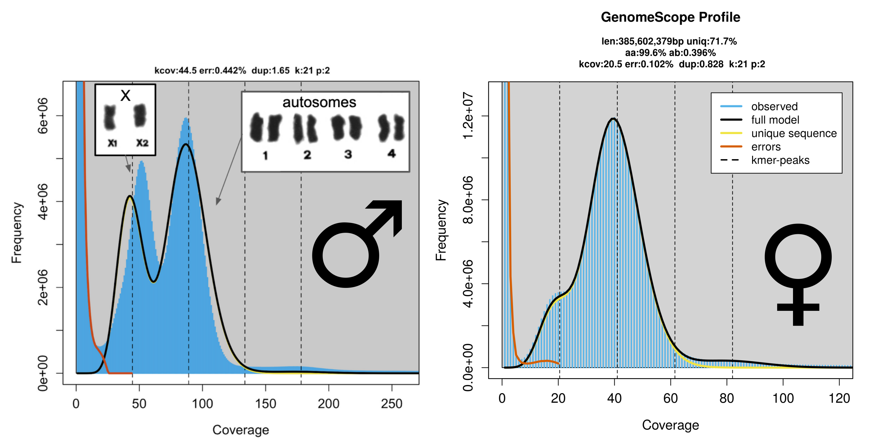
Here we are looking at the k-mer spectra of male and female globular springtail. In this species males have two chromosomes haploid (X) and 4 chromosomes diploid (autosomes), which is the reason why the 1n peak is so large. Females have all the chromosomes diploid and the small 1n lump is really the heterozygsity.

Note that the genome size and heterozygsity estimates are erased in the male model because they are completelly meanlinless as the basic assumpation of the same ploidy of all chromosomes is violated.

plotting 1d k-mer spectra

exercise

1. For sample1 assigned to your group create k-mer spectra and a k-mer dump (will be needed later). You already know how to build a KMC database and extract the histogram, but if not, here is reminder.

2. Extract alphabetically sorted k-mer dump from the database from a "reasonable coverage" range.

You can extract the dump from the same database as the histogram. You need to specify the coverage range (-ci and -cm parameters). Without seing the data, I would suggest to use -ci5 (mostly error k-mers) and -cm300 (we care mostly about monoploid or diploid k-mers anyway). Finally, to get the dump alphabetically sorted, you need to specify parameter -s.

kmc_tools transform <kmcdb> -ci<min_cov> -cx<max_cov> dump -s <output_name.dump>

What do you think by looking at the kmer spectra, do you have a male or female? One of your group should post the k-mer spectra to #session-2-separating-chromosomes on slack.

Save the coreesponding dump to /cluster/projects/nn9458k/oh_know/teachers/kamil/data/tse-tse/dumps/Glossina_<sample>.dump, where <sample> will be the corresponding sample number.

solution

For Glossina_12

cd $USERWORK

# create new working dir and some directories to keep it a bit tidy
mkdir -p tse-tse/reads tse-tse/scripts tse-tse/kmer_db tse-tse/genomescope
cd tse-tse/


# copy (again) the scripts, and symlink your input files
cp /cluster/projects/nn9458k/oh_know/teachers/kamil/data/genome_characterisation/*sh scripts
ln -s /cluster/projects/nn9458k/oh_know/teachers/kamil/data/tse-tse/Glossina_12_R[1,2].fastq.gz reads

# build kmer database (this will take a longer moment for this sized dataset)
ls reads/Glossina_12_R[1,2].fastq.gz > reads/read_files
sbatch ./scripts/build_KMC_db.sh reads/read_files kmer_db/Glossina_12

# extract k-mer dump (we will need it later on). This step will take a moment, but next two steps (plotting 1d and 2d spectra) do not depend on it, so you can carry on
sbatch ./scripts/create_kmer_dump_kmc.sh kmer_db/Glossina_12 5 300 kmer_db/Glossina_12_k21_L5_U300.dump
cp kmer_db/Glossina_12_k21_L5_U300.dump /cluster/projects/nn9458k/oh_know/teachers/kamil/data/tse-tse/dumps/Glossina_12.dump

# get histogram
sbatch ./scripts/get_histogram.sh kmer_db/Glossina_12 genomescope/Glossina_12_k21.hist

# fit genomescope model (default diploid will do for getting an idea)
sbatch ./scripts/fit_genomescope.sh genomescope/Glossina_12_k21.hist genomescope Glossina_12 2

plotting 2d k-mer spectra

2d k-mer spectra is in principle the same thing as k-mer spectra. But instead of counting the k-mer coverage of a k-mer in one reads set, we calculate it in both sets of sequencing reads. Then the plot won't be a histogram, but a 2d density plot, where two axis are coverages in respective libraries and the intensity of colour indicate the frequency of k-mers for every combination of coverages.

exercise

3. plot 2d k-mer spectra of your Glossina samples (each group has two assigned, see table at the top)

This plot can be made using KAT, which is a very handy tool for manipulating k-mers and we will use it several times over this workshop. To use KAT, you need to load module module add KAT/2.4.2-foss-2019a-Python-3.7.2. KAT has many functionalities, but comparing of two libraries done by comp module.

kat comp -n -t 16 -o <output_prefix> '<sample_1_reads_F.fastq.gz> <sample_1_reads_R.fastq.gz>' '<sample_2_reads_F.fastq.gz> <sample_2_reads_R.fastq.gz>'

this command generates a .mx file (a 2d equivalent of .hist), but also a .png plot with the visualized histogram. If you would like to replot the 2d histogram you can use the following function (without a need to recalculate the .mx file)

kat plot density <matrix_file>

Here is an example of two globular springtails shown above

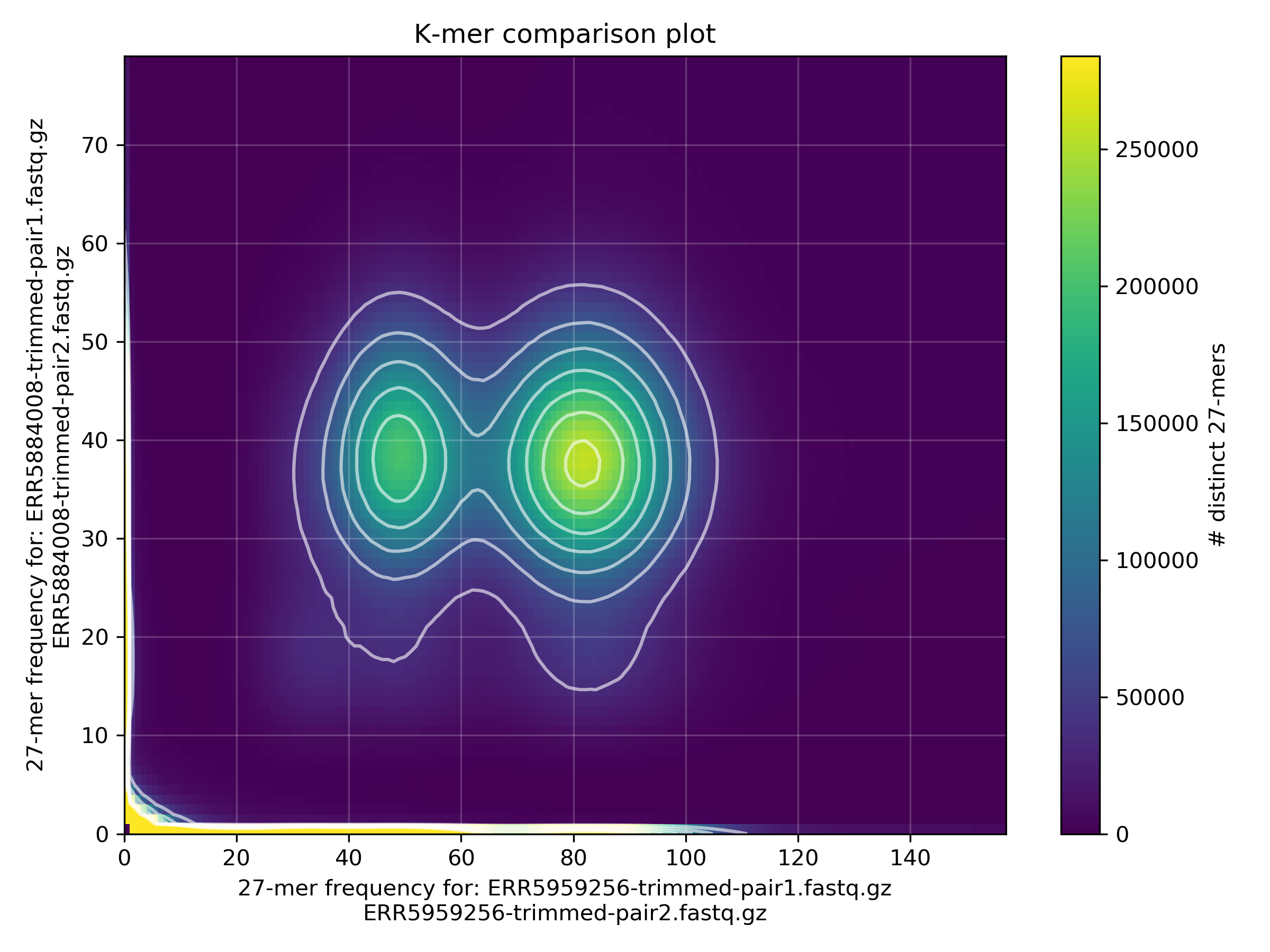
We can clearly see

• k-mers that are 1n in males and 2n in females (X-linked)
• k-mers that are 2n in both males and females (A-linked)
• k-mers that are clearly errors
• k-mers that are specific to the two individuals (reflecting genetic diversity of the species)

Now, gene generates 2d k-mer spectra for sample1 and sample2 of assigned to your group.

Can you tell which k-mers are which? What do you think, do tse-tse flies have Y chromosomes?

pause for the disucssion: Let's together fill sex of the samples in the following table: /cluster/projects/nn9458k/oh_know/teachers/kamil/data/tse-tse/tse-tse_sample_table.tsv.

solution

again for Glossina_12 and Glossina_14, assuming presence of the files from the last solutions.

# link also the other sample
ln -s /cluster/projects/nn9458k/oh_know/teachers/kamil/data/tse-tse/Glossina_14_R[1,2].fastq.gz reads
mkdir kat

# submit a script that execute kat comp -n ...
sbatch ./scripts/kat_for_libraries.sh reads/Glossina_12 reads/Glossina_14 kat/Glossina_12_vs_14

2. Extracting k-mers matching certain criteria

Now, that we know how to make the 2d k-mer plot, let's find chromosome-specific k-mers. As no one has actually seen the tse-tse data, we can't write here what threshold we should use, that's something we will need to discuss together dependent on the results of the previous section.

determining thresholds

To show you how the thresholds can be terminted, here we show an example of Bradysia tilicola from Hodson et al. 2021. In this preprint, germ-line restricted chromosomes were isolated by comparing a library made of testes and heads of flies. The karyotypes in the two types of tissues, as well as 2d k-mer spectra, are in the figure 1 from the manuscript

Hence for the isolation of 27-mers corresponding to X, GRC or autosomes respectively we chose the following thresholds (boxed on the image)

A
 - 125 < head   < 175
 - 80  < testes < 140
X
 - 50  < head   < 100
 - 60  < testes < 100
GRC
 - head < 5
 - 15 < testes # this might be too stringent

So, let's decide the thresholds for each library in the tse-tse data. I had no way to know the answer when I was writing this tutorial, hence we really have to figure it out together.

pause for the disucssion: And let's write together thresholds /cluster/projects/nn9458k/oh_know/teachers/kamil/data/tse-tse/tse-tse_sample_table.tsv

extracting k-mers

As far as I can tell, there is no native tool that would fish out the k-mers for us (though I would not be surprised if there was one, or if there will one implemented soon). However, we can work around it by merging k-mer dumps.

exercise

4. merge all k-mer dumps together into one file with sample coverages at solumns.

Hopefully, we already have extracted dumps of kmers using kmc. We have a bash script that reads the 8 dump files simultaneously and merges the coverage information in a format as follows

kmer	sample1	sample2	sample3	...	sample8
ATTCAT	54	72	3	..	43
AGCGGC  24	1	15	..	23
...

The syntax of the script is as follows

merge_dumps.sh <path/to/1.dump> <path/to/2.dump> ... > tse-tse_merged_dumps.tsv'

The script is using bash utility join for merging the files by the first row. It's nothing very sophisticated, I will try to run it once we will have all files, so you can use the file I am going to generate - /cluster/projects/nn9458k/oh_know/teachers/kamil/data/tse-tse/tse-tse_merged_dumps.tsv.

And now, using the thresholds we have decided on above, we generate kmer fasta files using another python script. This one is a bit tricky, normally I would write the coverage thresholds and sexes of samples right away in the script, but in this case, I knew nothing of it. Hence, I write a script dump2fasta.py takes the dump as one argument, but also the sample table /cluster/projects/nn9458k/oh_know/teachers/kamil/data/tse-tse/tse-tse_sample_table.tsv with all the per-sample sexes and coverage thresholds. It is expected to be read from the table <sample_table.tsv>, which is just a tsv file, with sample sex monoploid_min monoploid_max diploid_min diploid_max columns and rows with the corresponding sample names as they appear in the dump files.

python3 dump2fasta.py <merged.dump> <sample_table.tsv> <output_pattern>

I would like to disclaim that I am not sure how long it will take, as I was testing the script using only dummy files (and I don't think it is particularly efficiently written). I would also like to encourage you to play with the script - you can change the thresholds, or the selection criteria (I decided to pick a k-mer as assigned to a chromosome if it had the expected ploidy in at least 3 males and 3 females).

Finally, for your own project, I heavily recommend exploring the data first before deciding on the selection criteria. Check how consistent are "Y-looking" or "X-looking" kmers in different male samples. You might discover a crucial piece of puzzle that will help you in figuring out what's going on.

solution

This was NOT tested, as I had no all the dumps at the disposition. However, it was tested with a dummy dataset, in principle it should work :-).

cd $USERWORK

# this part will be easier in an interactive mode as nothing is paralelized or really very computationally heavy
srun --ntasks=1 --mem-per-cpu=10G --time=01:00:00 --qos=devel --account=nn9458k --pty bash -i

# get the dump files of other groups
ln -s /cluster/projects/nn9458k/oh_know/teachers/kamil/data/tse-tse/dumps/ .
ls dumps/*.dump | wc -w # is it 8? if it's not, we need to find the remaining file(s)
# get the hopefully fille sample table
cp /cluster/projects/nn9458k/oh_know/teachers/kamil/data/tse-tse/tse-tse_sample_table.tsv .

# merge dumps into one
merge_dumps.sh dumps/*dumps > dumps/tse-tse_merged_dumps.tsv'

# make sure the sample table is filled right
cat tse_sample_table.tsv
# does it look like it's filled with values (the temple file had all samples with M/F	5	15	15	25 values)

python3 dump2fasta.py dumps/tse-tse_merged_dumps.tsv tse_sample_table.tsv tse-tse-kmers-chr
# should generate 3 files - _X.fa _A.fa and _Y.fa

3. Matching k-mers to a genome

Here we want to find exact matches of k-mers in the genome assembly. We can tweak a fast popular mapper bwa mem to do so (thanks to Daniel Standage for the tip) by setting up minimum seed length -k (the initial match required to consider mapping) as well as the minimum score to output -T to the value k we used. We also specify -a as we want all the matches (although we don't expect to see many of those). -c just skips all seeds (k-mers) with more than hits than the value specified (5000 in the example)

bwa mem -k <k> -T <k> -a -c 5000 <assembly.fasta> <kmers.fasta>

The lates Glossina assembly is downloaded from NCBI here: /cluster/projects/nn9458k/oh_know/teachers/kamil/data/tse-tse/ncbi-genomes-2021-09-12. The mapped bams can be summarised into a table of scaffolds with the number of k-mers from each category. To do that we will use another home-made script, bams2table.py:

python3 bams2table.py <A_kmers_mapped.bam> <X_kmers_mapped.bam> <Y_kmers_mapped.bam> <output_per_scf_table.tsv>

Finally, now <output_per_scf_table.tsv> contains names of all scaffolds and number of chromosome specific k-mers. Just looking at the table... Q: did the assembly contain Y? Q: What is the longest clearly X-linked scaffold? The signal is usually clear, but hardly ever perfect. What causes that k-mers assigned to all three chromosomes map to so many scaffolds? Can we find any probably chimeric scaffold?

If there will be enough time, we can plot the properties of mapped k-mers and decide on scaffolds that can be clearly assigned to chromosomes and actually generate a table of assignments. Do you have an idea to get the Y chromosome too?

4. Matching k-mers to sequencing reads

The other option to utilize the chromosome-specific k-mers is to extract them from reads. Of course, at this point, you probably know enough about kmers to find some sort of way to match k-mers to reads too, but fortunately, for this, there is an existing tool - Cookiecutter (Thanks Rob Baird for this pointer).

Cookiecutter is a command-line tool, that allows to subset reads to those that do or don't specified k-mers.

python2.7 cookiecutter make_library -i <Y-kmers.fasta> -o <Y-kmers.lib.txt> -l <k>
python2.7 cookiecutter extract -1 <reads_R1.fq> -2 <reads_R2.fq> -f <Y-kmers.lib.txt> -o <Y_reads>

The extracted reads are those that contain at least one of the specified k-mers. The utility also allows to exclude reads that contain a specified k-mers, therefore one can subsequently subset the extracted reads to those that contain Y-linked k-mer only

python2.7 cookiecutter make_library -i <A-kmers.fasta> <X-kmers.fasta> -o <AX-kmers.lib.txt> -l <k>
python2.7 cookiecutter remove -1 <Y_reads.fq> -2 <Y_reads.fq> -f <AX-kmers.lib.txt> -o <Y_reads>

The reads can be then assembled, or mapped back to an assembly.

5. Comparing mapping based and k-mer approaches

The other, by far more common, approach to identify individual chromosomes is via read mapping. The chromosomal assignet of reads is usually generated via log normalized male to female coverage ratio. In the already linked preprint about fungus gnats, panel B shows coverage ratios of head and testes libraries mapped on a genome assembly. With manually selected thresholds, the different peaks are associated with different chromosomes

In the manuscript, the GRC reliable assignments were made by agreement of the mapping and k-mer approach. However, one can imagine other ways how to combine the approaches, for example by comparison of mapped reads that were subset by k-mers as explained in the last section.

For chromosomes that are largely similar, these approaches are not so useful, where there are nearly no single copy chromosome-specific k-mers. That happens to be the case in songbird germ-line restricted chromosomes (see Kinsella and Ruiz-Ruano et al.; 2019 or ask Paco :-)). Look also at the paper for the chromosome assignments for these cases of extremely high sequence similarity. it's been also proposed by Asalone et al. 2021 to used a modified RNA-seq pipeline to detect the sequences that are shared between the studied chromosomes (GRCs in their case) and core genomes.