This repository contains the two Python3 toolboxes and a simple tutorial for the accompanying paper in Water Resources Research (current status: under review). If you want to gain some practical intuition for AEM, I have also created a simple interactive, web-based AEM model with an extraction well, an injection well, a no-flow boundary, and Möbius base flow. The model can be accessed here.
To use these toolboxes, simply download the Python files toolbox_AEM.py and toolbox_MCMC.py (if desired) and copy them into your working directory. The MCMC toolbox is optional and only required if you also wish to use my MCMC implementation, the AEM toolbox can work as a standalone. Both toolboxes can be imported into your Python script by including the following code snippet:
from toolbox_AEM import *
from toolbox_MCMC import *
And that's it!
I have provided a few simple tutorials to help you familiarize yourself with the toolbox. The basic tutorial covers the fundamentals of constructing a deterministic flow model with this toolbox, and is available as both a Python file and a Jupyter Notebook.
The advanced tutorial expands the scope of the basic tutorial by showing how to prepare the Analytic Element Model for uncertainty quantification. This tutorial is also available as both a Python file and a Jupyter Notebook.
For users with an interest in reproducing the some or all of the results in accompanying manuscript, I have also uploaded the Python files required to reproduce the figures in the main manuscript and the supporting information.
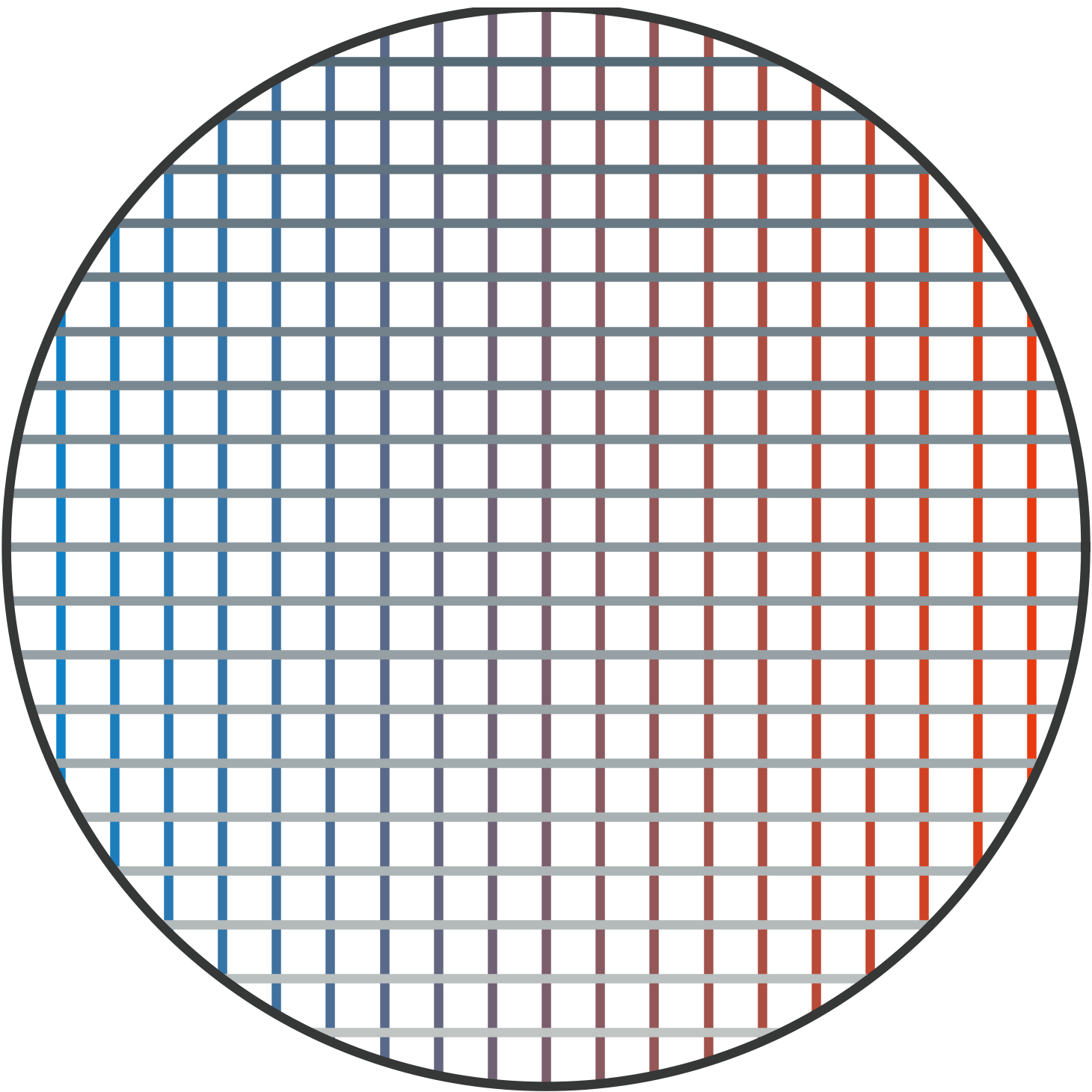
To provide a background potential or unidirectional regional flow, the simplest option is to use uniform flow, specified by the AEM toolbox' object ElementUniformBase. This element requires the specification of a direction in radians, a minimum and maximum hydraulic head, and a background hydraulic conductivity.
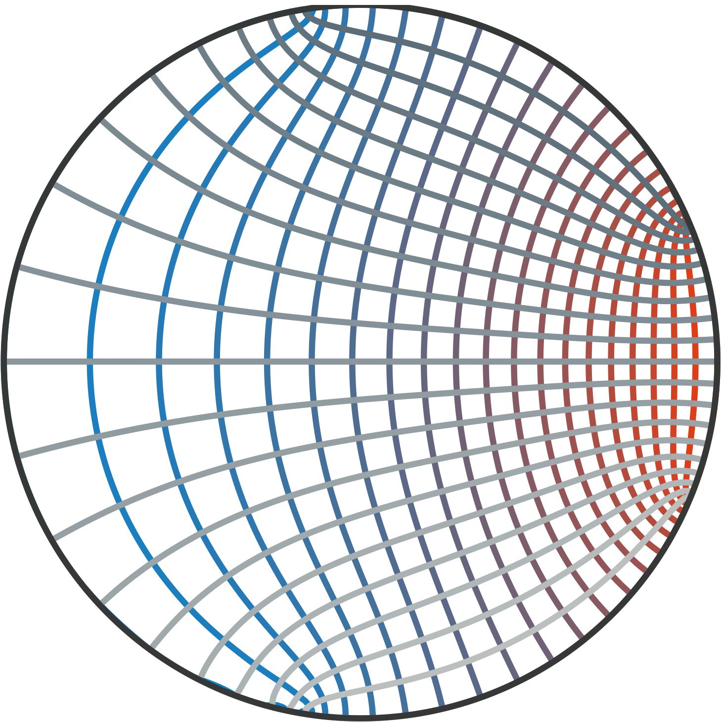
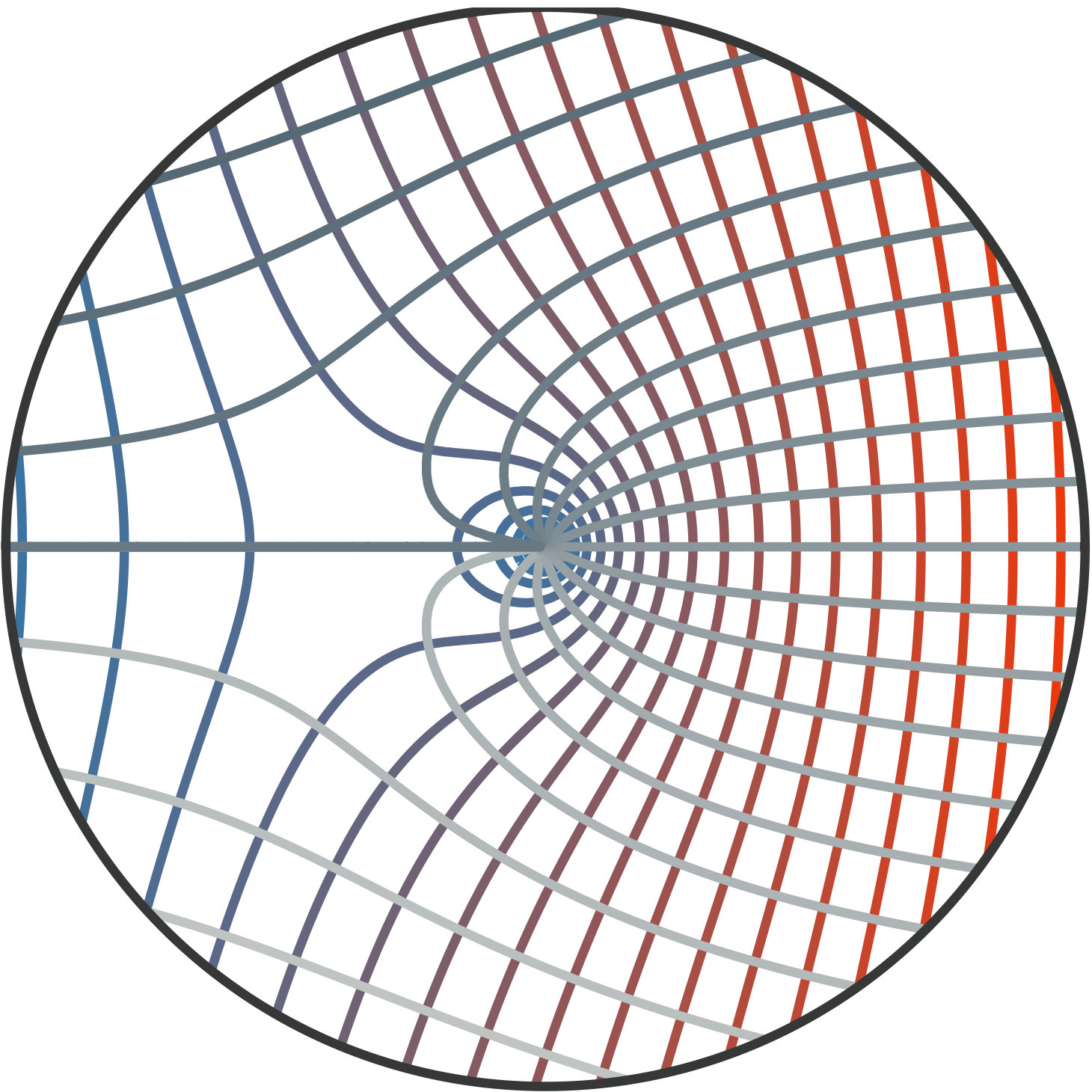
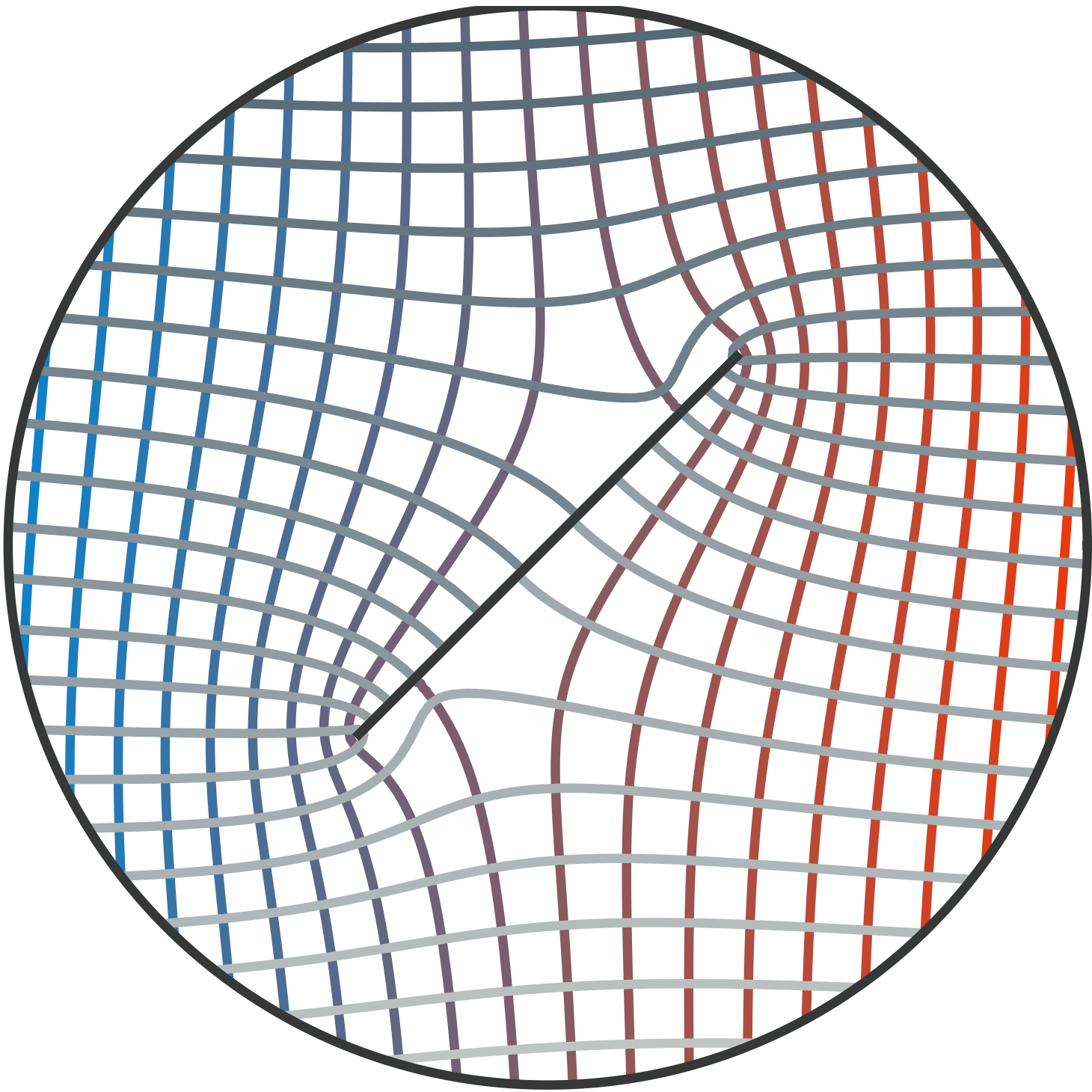
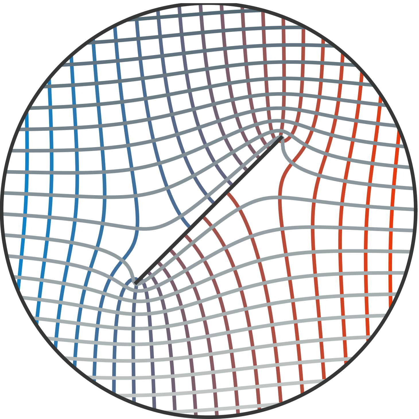
Möbius base flow provides a way to implement more intricate regional flow, allowing for curvature, divergence, and convergence. This type of flow is specified by the AEM toolbox' object ElementMoebiusBase. This element requires the specification of three control points' direction in radians, a minimum and maximum hydraulic head, and a background hydraulic conductivity.
Injection or extraction wells - or any other type of pointwise flow - can be implemented using the ElementWell object. This element requires the specification of a position, a positive or negative strength value, and a well radius. Alternatively to a strength value, this element can also adjust its strength to induce a desired drawdown on the flow field.
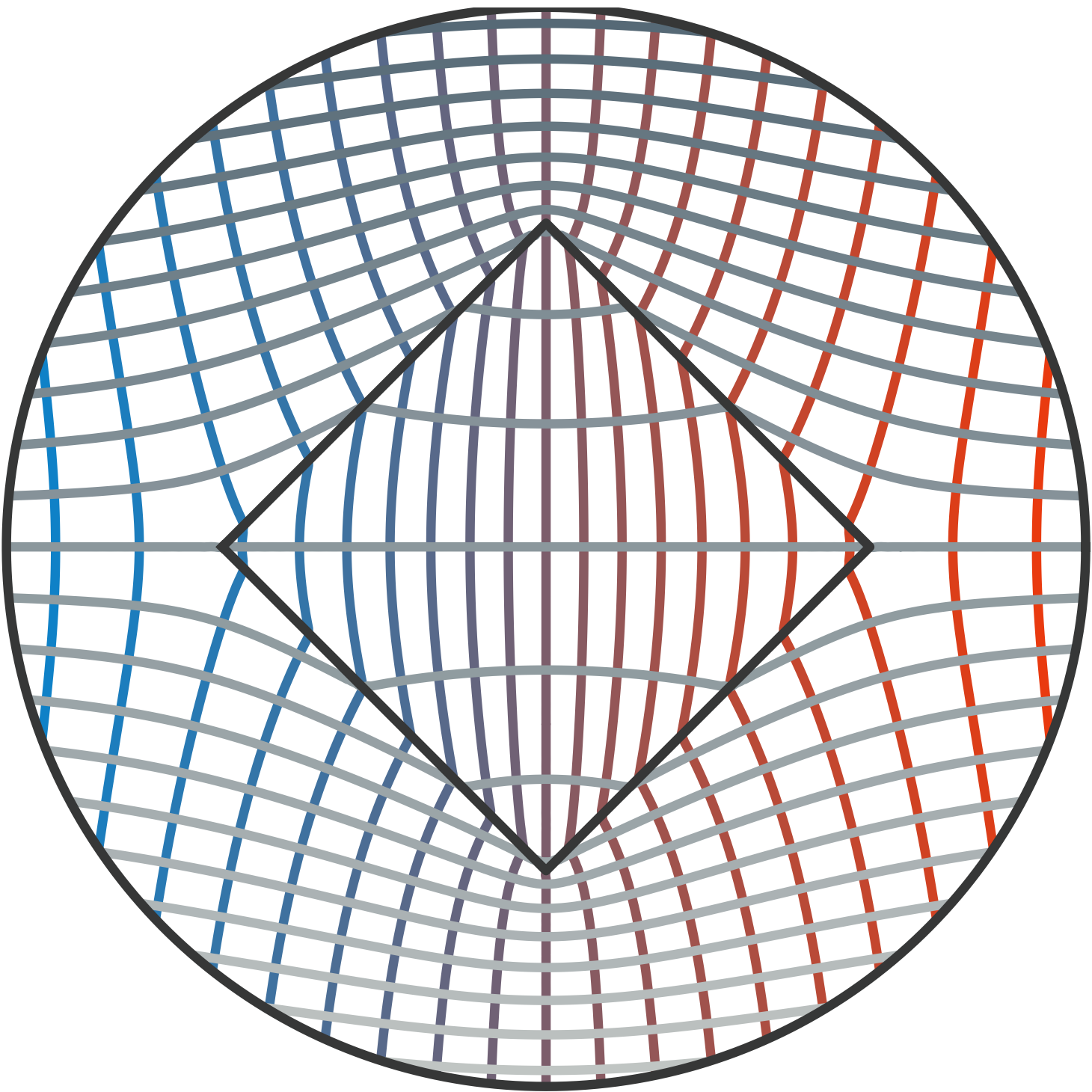
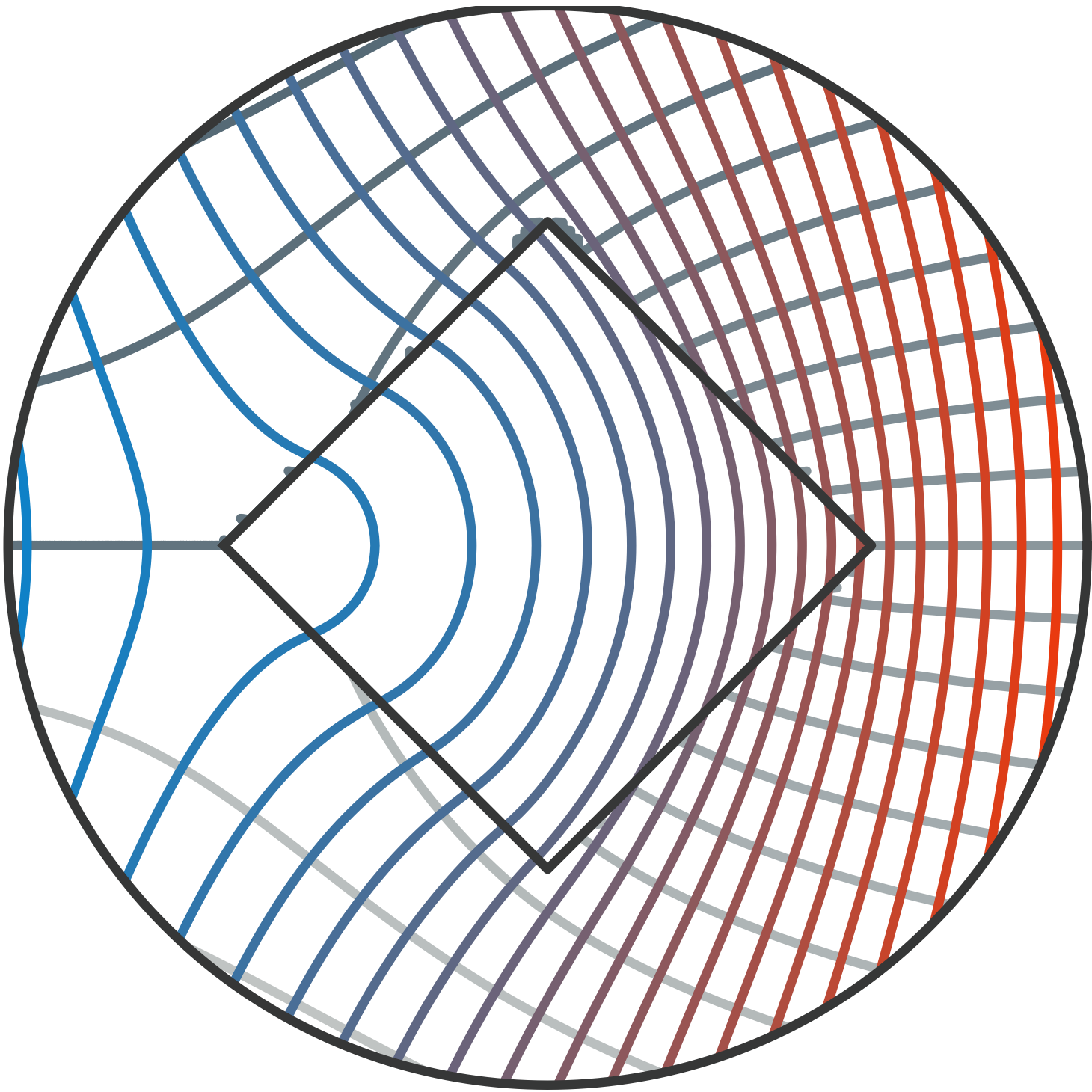
Zonal inhomogeneities in the aquifer's hydraulic conductivity can be represented using the ElementInhomogeneity object. This element requires the specification of a hydraulic conductivity value, as well as a closed or open polygon defining its extent.
Prescribed head boundary conditions or rivers can be created using the ElementHeadBoundary object. This line element enforces a specified hydraulic head along its path. It requires the specification of its vertices and corresponding head values. It also allows for the implementation of a uniform or spatially varying connectivity value which can limit its influence on the water table.
No-flow boundaries from sheet pile walls or impermeable formations can be created using the ElementNoFlowBoundary object. This line element requires only the specification of the vertices along its path and can be either closed or open.
Areal recharge or water extraction can be represented using the ElementAreaSink object. This element adds or removes water according to a specified range inside its polygon. It requires the specification of its polygons and a positive or negative strength value. Not that the stream function component of the complex potential is not valid inside an area source or sink.
Q: The model seems to create singularities, predicting very high or low water tables at certain isolated locations. What did I do wrong?
A: This usually happens if the model attempts to evaluate the complex potential Ω directly on an element. This can happen because because two elements share a line segment or because one of the evaluation points lies on an a line segment. Make sure that the elements do not share direct borders, for example by offsetting them by a minuscule amount (e.g., 1E-10). I have implemented protections against this for some but not all elements: inhomogeneity elements, for example, are automatically shrunk by a negligible amount. Also, you should make sure that no inhomogeneities or no-flow boundaries intersect.
Q: There are still strange artefacts along my no-flow boundaries or inhomogeneities. What happened?
A: If you have tried the solutions in the answer above and the issue persists, try increasing the resolution of the element by increasing the element's segments. Most of the constant-strength line elements I used here require sufficient resolution to induce the desired effect. It is difficult to predict how large this resolution should be in advance.
Q: Why are there discontinuities in the stream function away from my wells, head boundaries, or area sinks?
A: These are so-called branch cuts, discontinuities in the stream function (the imaginary part of the complex potential) which arise whenever an element adds or removes water from the system. An example can be seen in the last image created in the basic tutorial. Unfortunately, there is no way to avoid them. For particle tracking purposes (when using the stream function, not the hydraulic potential), I advise capitalizing on the fact that these branch cuts occur in predictable patterns and explicitly account for them in your tracking routine. For plotting purposes, I recommend not using ready-made contouring functions, but instead plotting the streamlines with with a particle tracking routine.
Q: The stream function appears discontinuous between the inside and outside of my area source or sink. Why?
A: The stream function is not valid inside of area sinks or sources. If you want to plot the stream function anyways, I recommend masking the stream function inside the area sink's or source's polygon, similar to what I did in the example area sink under the 'Elements' heading above.