Cortical reconstruction with MNE and MEM
This tutorial illustrates how to perform NIRS reconstruction using weighted Minimum Norm Estimate (MNE) and Maximum Entropy on the Mean (MEM).
Authors:
- Zhengchen Cai, PERFORM Centre and physics dpt., Concordia University, Montreal, Canada
- Thomas Vincent, PERFORM Centre and physics dpt., Concordia University -- EPIC Center, Montreal Heart Institute, Montreal, Canada
- Visual checkerboard task: 13 blocks of 20 seconds each, with rest period of 15 to 25 seconds
- One subject, one run of 17 minutes acquired with a sampling rate of 5Hz
- 2 sources and 10 detectors
- 2 wavelengths: 685nm and 830nm
- 3T MRI anatomy process by FreeSurfer 5.3.0 and SPM12
- you have already completed the brainstorm introduction tutorials #1 to #6 and the basic Nirstorm tutorial
- The nirstorm plugin has been installed.
- Download and uncompress the file: sample_nirs_reconstruction.zip. It contains a Brainstorm protocol file with NIRS data and anatomy for one subject, as well as pre-computed fluence data for the same subject in a separate folder.
- Start Brainstorm
-
From the menu of the Brainstorm main panel:
File > Load protocol > Load from zip file > Select the downloaded protocol file:
protocol_nirs_reconstruction.zip
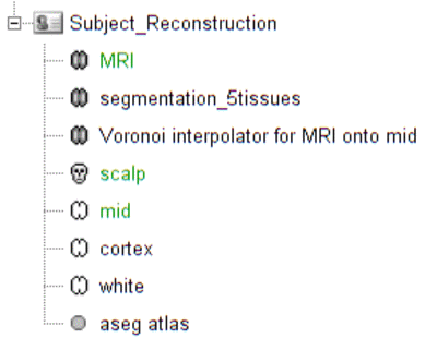
Switch to the "anatomy" view of the protocol. The anatomy data of subject Demo consists of:
- MRI: 3T MRI image of the subject
- Segmentation_5tissues: anatomical segmentation performed by FreeSurfer 5.3.0 and SPM12 tissues types contains scalp (labeled as 1), skull (labeled as 2), CSF (labeled as 3), gray matter (labeled as 4) and white matter (labeled as 5). In general, one could use segmentations calculated by other software. Note that the segmentation file was imported into Brainstorm as a MRI file, please make sure the label values are correct by double clicking on the segmentation file and reviewing by MRIViewer of Brainstorm.
- Voronoi interpolator for MRI onto mid: interpolators to project volumic data onto the cortical mid surface. It will be used to compute NIRS sensitivity on the cortex from volumic fluence data in the MRI space.
- scalp: scalp mesh calculated and remeshed by Brainstorm. To reduce the NIRS montage registration error, it is always better to remesh the head mesh so that two projected optodes do not end up on vertices that are too close.
- mid: mid-surface calculated by FreeSurfer 5.3.0 which is in the middle of the pial and white surface. This is a resampled version of the original file provided by freesurfer, with a lower number of voxels to reduce the computation burden of the reconstruction. The signal spatial resolution is quite coarse anyway so we don't need many vertices. 25000 vertices is a fine recommendation for MEM. Besides, note that the quality of this mesh is critical since it will the support of the reconstruction. Some mesh inconsistencies (crossing edges, non-manifolds, zero-length edges...) can occur during segmentation. See the last section of this tutorial to address this issue.
The anatomy view should look like:
** Make sure the default MRI, head mesh and cortical surface are the same as in this snapshot**
Please refer to this tutorial for details on how to perform pre-processings.
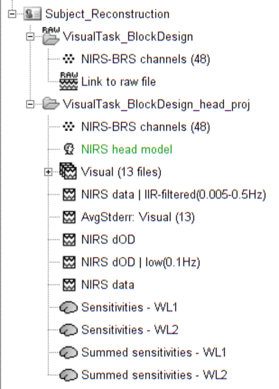
The functional view of the protocol should consist of:
-
VisualTask_BlockDesign: contains the raw acquisition data.
-
VisualTask_BlockDesign_head_proj: contains raw data that has been projected onto the scalp mesh ("NIRS > Project montage to head mesh").
Due to digitization and segmentation errors, optode positions may not match the scalp mesh. To fix this issue, they were projected to their nearest vertex on the scalp mesh. Note that the montage registration could have be done more accurately by the Brainstorm process "Refine registration with head points". This process requires at least 100 digitized head points.
-
VisualTask_BlockDesign_head_proj: contains pre-porcessed data:
- NIRS-BRS channels (48): NIRS channel file
- NIRS data: imported raw NIRS data
- NIRS data | IIP-filtered(0.005-0.5Hz): band-pass filtered raw data in between 0.005 and 0.5 Hz. This process should remove any low frequency drift.
- NIRS dOD: delta optical density (obtained by normalizing raw data and applying log)
- NIRS dOD | low(0.1Hz): low-pass (0.1Hz high cut-off) filtered dOD to remove cardiac and respiratory artifact
- Visual (13 files): 13 block trials exported from NIRS dOD | low(0.1Hz) with a window size of -10 seconds to 40 seconds
- AvgStderr Visual (13): block-average of visual trials (13 files), with standard error. This data trial will be the input of the reconstruction.

The NIRS reconstruction process relies on the so-called forward problem which models light propagation within the head. It consists in generating the sensitivity matrix that maps the absorption changes along the cortical region to optical density changes measured by each channel (Boas et al., 2002). Akin to EEG, this is called here the head model and is already provided in the given data set. We refer to this tutorial (TODO) for details about head model computation.
The visualize the current head model, first let's look at summed sensitivities which provide an overall cortical sensitivity of the NIRS montage. To go into more details, the head model can be explored channel-wise. Double click Sensitivites - WL1 and Sensitivites - WL2. We used a trick to store pair information in the temporal axis. The two first digits of the time value correspond to the detector index and the remaining digits to the source index. So t=101 corresponds to S1D1. With the same logic, t=210 will be used for S2D10. Note that some time indexes do not correspond to any source-detector pair and the sensitivity map will then be empty. The following .gif figure shows the summed sensitivity profile of the montage (top) and the sensitivity map of each channel (bottom).

TODO: create other tutorial on MCXLAB / forward model computation and refer to it
Forward model computation requires a well-segmented head which contains five tissue types (i.e. scalp, skull, CSF, white matter and gray matter) and the optical proprietaries (i.e. absorption and scatting coefficient) of each tissue. Fluences of light for each optode (i.e. source and detector) was estimated by Monte Carlo simulations using MCXLAB developed by (Fang and Boas, 2009, http://mcx.space/wiki/index.cgi?Doc/MCXLAB). Sensitivity values in each voxel of each channel were computed by multiplication of fluence rate distributions using the adjoint method according to the Rytov approximation as described in (Boas et al., 2002). Nirstorm can call MCXLAB and calculate the fluences for each optode. To do so, one has to set the MCXLAB folder path in matlab and has a dedicated graphics card since MCXLAB is running by parallel computation using GPU. Don worry, the sample package in this tutorial already contains all of the fluences files calculated by the first step as following. If you are not able to run MCXLAB, just skip the first step.
- Drag and drop "AvgStderr Visual (13)" into the process field and press "Run". In the process menu, select "NIRS > Compute fluences for optodes by MCXlab". Enter the fluences output path as set the parameters as the
following snapshot. All these parameters are described in detail on http://mcx.space/wiki/index.cgi?Doc/README The important ones are cfg.gpuid which indicate which GPU one would like to use for calculation and cfg.nphoton which assigns the number of photon will be launched in the Monte Carlo simulations. The fluences data included in this package were calculated using 10^{8} photons. If you have multiple GPUs, it is always better to use the one that is not working for displaying purpose. **Swep GPU **allows users to launch the computation one GPU by another only when the cooling system is not able to maintain a good temperature for graphic card during heavy computations. To reduce the output file size, one could check the "Set threshold for fluences" and specify the threshold value. {{..\Figure_NIRS_Reconstruction\Screenshot from 2018-04-03 14-50-50.png}}- Drag and drop "AvgStderr Visual (13)" into the process field and press "Run". In the process menu, select "NIRS > Compute head model from fluence". Copy and paste the fluences file path into the **Fluence Data Source. **Checkbox "Mask sensitivity projection in gray matter" allows to only project the sensitivity values within gray matter to the cortex surface. "Smooth the surface based sensitivity map" will spatially smooth the sensitivity arrording to the FWHM value. After running this process, a NIRS head model file called "NIRS head model from fluence" will be showed in the functional folder. Note that in Nirstorm, the sensitivity values within the gray matter volume were be projected onto the cortical surface using the Voronoi based method proposed by (Grova et al., 2006). This volume to surface interpolation method has the ability to preserve sulco-gyral morphology. After the interpolation, the sensitivity value of each vertex of the cortex mesh (default mesh in the anatomical view of Brainstorm) represents the mean sensitivity of a corresponding set of voxels that have closest distances to a certain vertex than to all other vertices. {{..\Figure_NIRS_Reconstruction\Screenshot from 2018-04-03 14-52-17.png}}{{..\Figure_NIRS_Reconstruction\Screenshot from 2018-04-03 14-54-15.png?height=408}} To visualize the sensitivity or head model on the cortical space, one need to Drag and drop "AvgStderr Visual (13)" into the process field and press "Run". In the process menu, select "NIRS > Extract sensitivity surfaces from head model".
Reconstruction amounts to an inverse problem which consists in inverting the forward model to reconstruct the cortical changes of hemodynamic activity within the brain from scalp measurements (Arridge, 2011). The inverse problem is ill-posed and has an infinite number of solutions. To obtain a unique solution, regularized reconstruction algorithm are needed. In this tutorial, two reconstructions will be used: the Maximum Entropy on the Mean (MEM) and depth weighted Minimum Norm Estimate (MNE).
Minimum norm estimation is one of the most widely used reconstruction method in NIRS tomography. It minimizes the l_{2}-norm of the reconstruction error, ie Tikhonov regularization (Boas et al., 2004b).
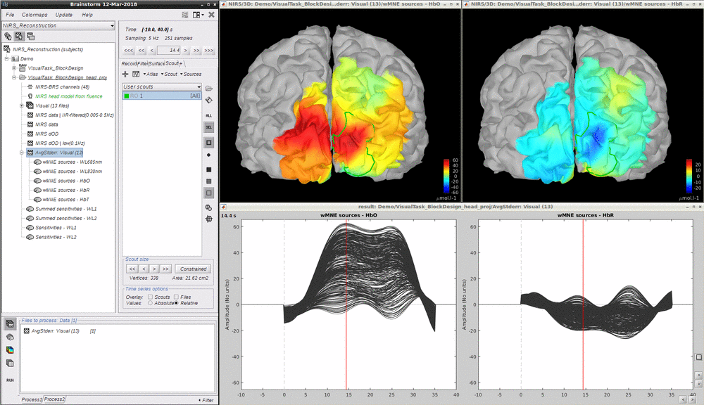
Drag and drop "AvgStderr Visual (13)" into the process field and press "Run". In the process menu, select "NIRS > Source reconstruction - wMNE.
Parameters are as follows:
- Reconstruction Field of view (distance to montage border) defines the "Field of view" of the reconstruction. Since NIRS montage usually only covers part of the brain, it is not necessary to preform reconstruction to the whole brain. This field of view is defined by the distance between 100% inflated cortex sruface and the border of the montage on the head mesh (outline of all the optodes).
- Depth weighting factor for MNE defines how much depth weighting one would like to set within the rang of [0 1]. The higher the value is the deeper the reconstruction would go. We highly recommend to use 0.5. NIRS is a technique that can only detect hemodynamic activities within superficial regions of the brain. Depth weighting in NIRS reconstruction is mainly to somehow compensate the fact that NIRS sensitivity decrease exponentially to the depth and the reconstruction favors only very superficial regions without any depth weighting.
- **Start and end time of the reconstruction **: defines the portion of the input signals to actually reconstruct on the cortex.
- Compute noise covariance of the baseline MNE: flag to compute the covariance on a portion of the input signal which is assumed background noise, called "baseline" here. If unchecked, identity matrix will be used to model the noise covariance.
- Start and end time of the baseline: defines the portion of the input signal to take as baseline (taken into account only if previous checkbox is checked).
- Store sparse result: in-dev feature (leave unchecked).
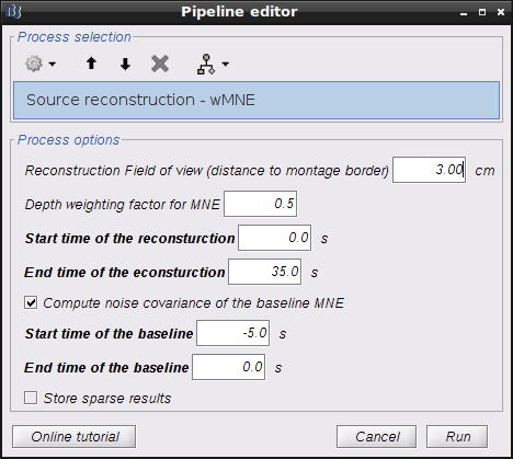
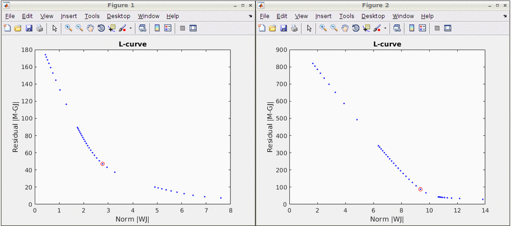
Note that standard L-Curve method (Hansen, 2000) is applied to optimize the regularization parameter in MNE model. This actually needs to solve the MNE equation several times to find the optimized regularization parameter so that it will take around 8 minutes to finish. Two L-Curves will be plotted right after the calculation. And the reconstruction results will be listed under "AvgStderr Visual (13)". Reconstructed time course can be plotted by using the scout function as mentioned in MEM section.
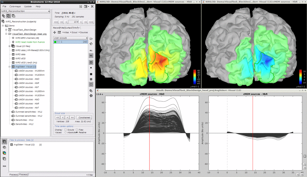
Maximum Entropy on the Mean (MEM) framework was first proposed by (Amblard et al., 2004) and then applied and evaluated in Electroencephalography (EEG) and Magnetoencephalography (MEG) studies to solve inverse problem for source localization (Grova et al., 2006; Chowdhury et al., 2013). We have adapted, improved and evaluated NIRS reconstruction using MEM. Using realistic simulations and well-controlled finger tapping data, we demonstrated excellent accuracy and stability of DOT using MEM, when recovering the locations of the underlying hemodynamic responses together with their spatial extent along the cortical surface. Please refer to this tutorial for more details on MEM. Note that performing MEM requires the **BEst – "Brain Entropy in space and time" **package which is included in the Nirstorm package.
- Drag and drop "AvgStderr Visual (13)" into the process field and press "Run". In the process menu, select "NIRS > Source reconstruction - cMEM".
Depth weighting factor for MNE and Depth weighting factor for MEM 0.5 for wMNE and 0.3 for MEM in most of the cases. If needed, only tune the MEM one to be lower values for deeper regions.
Set neighborhood order automatically. This will automatically define the clustering parameter (neighborhood order) in MEM. Otherwise please make sure to set one in the MEM options panel during next step.

- Select "cMEM" in the "MEM options" panel. Keep most of the parameters by default and set other parameters as following:
- Data definition > Time window: 0-35s which means only the data within 0 to 35 seconds will be reconstructed
- Data definition > **Baseline > within data > Window: **-5-0s which defines the baseline window that will be used to calculate the noise covariance matrix in MEM
- Clustering > Neighborhood order: If "**Set neighborhood order automatically" **is not checked in the previous step, please give a number such as **"8" **for NIRS reconstruction. This neighborhood order defines the region growing based clustering in MEM framework. Please refer to this tutorial for details. If "**Set neighborhood order automatically"**is checked in the previous step, this number will not be considered during MEM computation.
- CPU parallel computation is allowed in MEM computation. To do so, click Expert and check Matlab parallel computing and make sure the parallel pool of Matlab is opened. This could save the time almost # of CPU cluster fold.
- After around 15 minutes, the resonstruction will be finished. Unfold AvgStderrL Visual(13) MEM reconstruction results will be showed. To check the reconstruction map, just double click the file such as "cMEM sources - HbO" and **"cMEM sources - HbO". **Multiple results using different parameters can be listed under the same file. Since the reconstruction of each wavelength was done independently, the reconstructed map of each wavelength was also available to check.
- To check the reconstructed time course of HbO/HbR, one need to manually define a scout region and set the **Scout function as "All", **select "Relative" in "Time series options > Values". This tutorial provides all the details about scout manipulation.
- Just for fun, please set the resampled surface as the default cortex and redo the analysis mentioned above. Of course the Compute Voronoi volume-to-cortex interpolator and the **Compute head model from fluence **have to be recalculated since the default cortex mesh has been changed. The comparison of the MEM reconstruction using the previous mid-surface (top) and the current one (bottom) is showed below. As one can see, the current one is smoother due the the fact that the mesh is more homogeneous. {{..\Figure_NIRS_Reconstruction\Screenshot from 2018-04-03 16-10-53.png?width=1200}}
TO CLARIFY
The cortical surface used in this tutorial was resampled from the original mid-surface calculated by FreeSurfer 5.3.0. One may know that the surface mesh calculated by FreeSurfer is not homogeneous and there might be self-intersecting triangular elements. NIRS reconstruction in Nirstorm is performing in surface space and some steps are related to the surface mesh quality such as the sensitivity projection using the Voronoi method and the cortex clustering in MEM. One could use the Brainstorm build-in function "Resample surface" by right-clicking on the original mid-surface (mid_262390V) and select one of the resampling options such as **iso2mesh **which can solve the problem of inhomogeneous and self-intersecting. By using this resampled cortical surface, we expected even better reconstruction results. {{..\Figure_NIRS_Reconstruction\Screenshot from 2018-04-03 16-22-12.png}}