Optimal montage
Author: ''Thomas Vincent, PERFORM Centre and physics dpt., Concordia University -- EPIC Center, Montreal Heart Institute, Montreal, Canada''
Reference article describing the methodology (pubmed):
Machado A, Marcotte O, Lina JM, Kobayashi E, Grova C., "Optimal optode montage on electroencephalography/functional near-infrared spectroscopy caps dedicated to study epileptic discharges". J Biomed Opt. 2014 Feb;19(2):026010.
TODO: add details on head scout (include / exclude regions) + precomputed region => create a dedicated page on the template and refer to it
TODO: propose heuristic to set nb of optodes wrt scout area
TODO: add export of coordinate file. Mention that is works well with brainsight neurovigation system
This process is part of the experimental planning, taking place before the acquisition, where the experimenter wants to define where to place the optode on the scalp. Usually, a NIRS montage has a limited coverage over the head and hence optodes are placed specifically on top of a predefined target cortical region of interest (ROI). However, due to the non-trivial light propagation across head tissues as well as the complex cortical topology, the optode placement cannot be optimally based solely on a pure geometrical criterion.
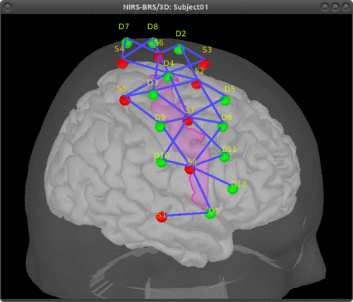
Here, the computation of the optimal NIRS montage consists here of finding the set of optode coordinates whose sensitivity to a predefined region of interest is maximized.
To achieve this, this process requires:
- an antomical MRI,
- pre-computed fluence data (see ...),
- a target ROI, either on the cortex or on the scalp.
For ease of configuration, the current tutorial relies on the Colin27 template adapted to NIRS Colin27_4NIRS. Indeed, fluence maps have already been pre-computed for this anatomy so that one can directly run the optimal montage process without going through the forward model computation. However, the most accurate results are obtained when using the subject-specific MRI. The current procedure can be straightforwardly transposed to any MRI.
- You have already followed all the brainstorm introduction tutorials #1 - #6 as well as the NIRS finger tapping tutorial,
- you have a working copy of Brainstorm installed on your computer.
- the nirstorm plugin has been downloaded and installed. See this page for instructions on installation.
- cplex version > 12.3 is installed, with matlab bindings available
- Get the template Colin27_4NIRS
- pre-computed fluence data is available for the current anatomy. For the template Colin27_4NIRS, fluence files are available online and will be downloaded automatically on-demand during the execution of the process.
- Start Brainstorm (Matlab scripts or stand-alone version)
- Select the menu File > Create new protocol. Name it "ProtocolOM" and select the options:
- "No, use individual anatomy",
- "No, use one channel file per acquisition run (MEG/EEG)".
- Create a new subject, eg "Subject1"
- Go to the anatomy view, right-click on Subject1 and select "Use template > Colin27_4NIRS"

For ease of reproducibility, the ROI definition is atlas-based. However, one can define its own ROI but building a custom cortical scout.
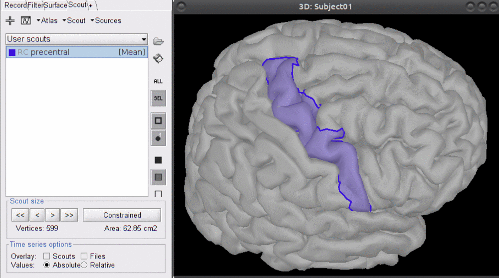
The first step is to define scout which represents the region of interest on which the sensitivity of the montage will be optimized.
- Open the mid cortical mesh by double-clicking on it in the anatomical view of subject1
- Select the scout panel and use the drop-down menu to show the Destrieux atlas
- Select the scout defining the right frontal transverse gyrus, labeled "RPF G_and_S_transv_frontopol".
- Click on Scout > export to matlab and name it "scout_frontal"
- Use the drop-down menu to show "User scouts"
- Click on Scout > Import from matlab and select "scout_frontal"
- Click on Scout > Rename and set the scout name to "scout_OM"
This ROI scout should end-up in the user-specific atlas "User scouts".
ADD SNAPSHOT
Note that this cortical scout comprises XXXX vertices and has an area of XXXX cm2. The scout size will matter while deciding how many sources and detectors to put in the montage.
The optimal montage works by searching for the best possible layout of optode pairings withing a given scout on the head mesh (search space). Each vertex in this head scout is a candidate holder on which an optode (source or detector) can be placed. A montage is the best if it maximizes the optical sensitivity over a pre-defined cortical scout (region of interest). Here, to avoid the explicit definition of the head scout (search space), we will use the process "Comoute optimal from cortex" which constructs the head scout by projecting the target cortical scout onto the head mesh. Alternatively, the head scout could be given explicitly while using the process "Comoute optimal from head".
Without using any data, click on RUN. Select process NIRS > Compute optimal montage from cortex. Here are the process parameters to fill, along with some explanation about them:

-
Extent of cortex-to-scalp projection: 2.5 cm
This is the maximum distance used to project the cortical scout onto the head mesh to create the head scout (search space). More precisely, a head vertex will be part of the projected head scout if it at most eg 3.OOcm away from the closest vertex in the cortical scout.
-
Cortical scout (target ROI): Subject1 > User scouts > scout_OM
It defines the target ROI on which the sensitivity is optimized.
The selector is experimental. It may not reflect the actual list of scouts. There may also be an error regarding scout selection during the execution of the process. To solve this, quit the process, and try to 1) callpanel_process_select('ParseProcessFolder',1)from the matlab prompt, 2) Reset process options (see snapshot below) 3) restart brainstorm.
Then restart the process again.
-
Output condition name: Optimal_Montage
The name of the condition which will contained the computed montage.
-
Wavelength (nm): 685
The wavelength of the fluence to load and which will be used to compute the optical sensitivity to the target cortical ROI.
-
Number of sources: 8
Maximal number of sources in the optimal montage. The actual number in the resulting montage may be lower. The recommendation is
-
Number of detectors: 12
Maximal number of detectors in the optimal montage. The actual number in the resulting montage may be lower. The recommendation is
-
Number of adjacent: 2
Minimal number of detectors that must be seen by any given source.
-
Range of optodes distance: 20 - 40 mm
Minimal and maximal distance between two optodes (source or detector). This applies to source-source and detector-dectector distances.
In short the optimal montage computations comprises the following steps with their typical execution time in brackets:
-
Mesh and anatomy loading [< 5 sec]
-
Loading of fluence files [< 2 min]
Fluence files will be first searched for in the folder .brainstorm/default/nirstorm/fluence. If not available, they will be requested from the resource specified previously (online here).
-
Computation of the weight table (summed sensitivities) [< 3 min]
For every candidate pair, the sensitivity is computed by summation of the normalized fluence products over the cortical target ROI. This is done only for pairs fulfilling the distance constraints.
-
Linear mixed integer optimization using CPLEX [< 5 min]
This is the main optimization procedure. It explores the search space and iteratively optimizes the combination of optode pairings while guaranteeing model constraints.
-
Output saving [< 5 sec]
** ADD SNAPSHOT **
Example with precentral gyrus.
ROI size:
Computation time: