instruments.sillyscope

Getting Started

mcphysics.instruments.sillyscope provides a scriptable graphical user interface for the sillyscopes commonly found in our student (and research) labs, including (but not necessarily limited to) Rigol B, D, E, and Z series, as well as many Tektronix models. To create a sillyscope instance,

import mcphysics
s = mcphysics.instruments.sillyscope()

This should pop up a window that looks something like this:

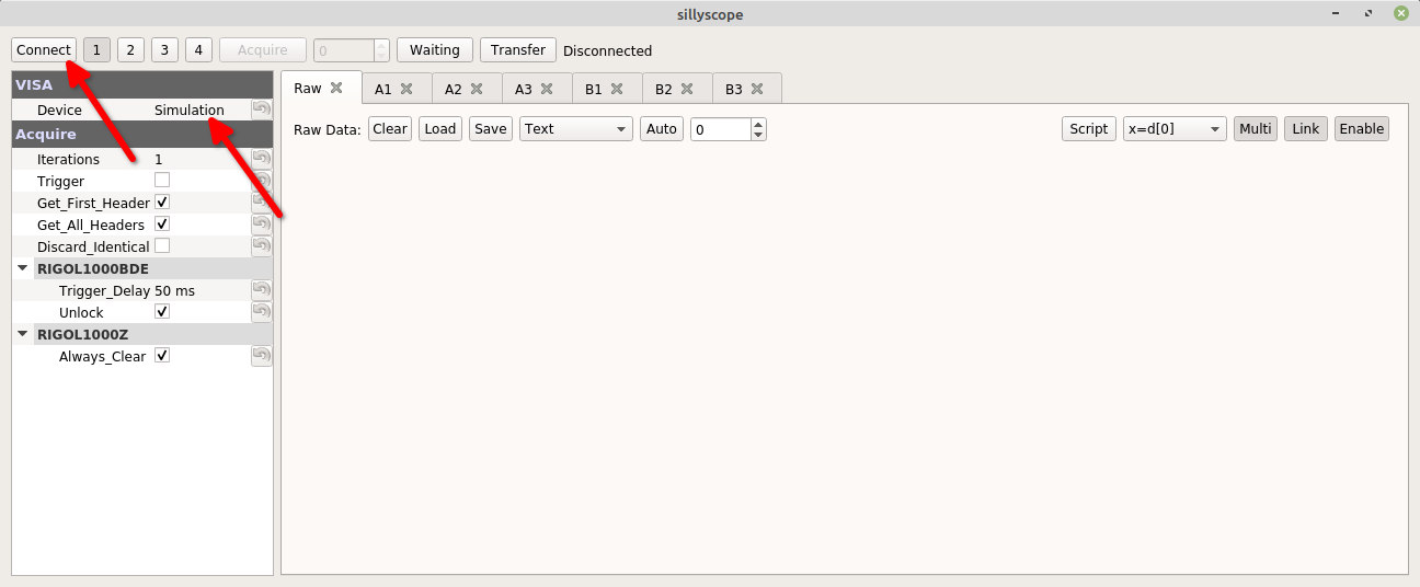
If you have a VISA driver + pyvisa installed (see Installation instructions), all connected instruments will appear in the "VISA/Device" menu. If they don't, you can try re-plugging them and closing / reopening all python consoles. Select the identifier associated with your scope and click the "Connect" button to connect. If it is successful, information about the device should appear at the top of the window. You may also select "Simulation" to test the scope interface without an actual scope connected. To collect data from the scope, select the relevant channels an click "Acquire". If it works, the data will be sent to the DataboxPlot object s.plot_raw in the "Raw" tab, which allows you to perform analysis on the fly:

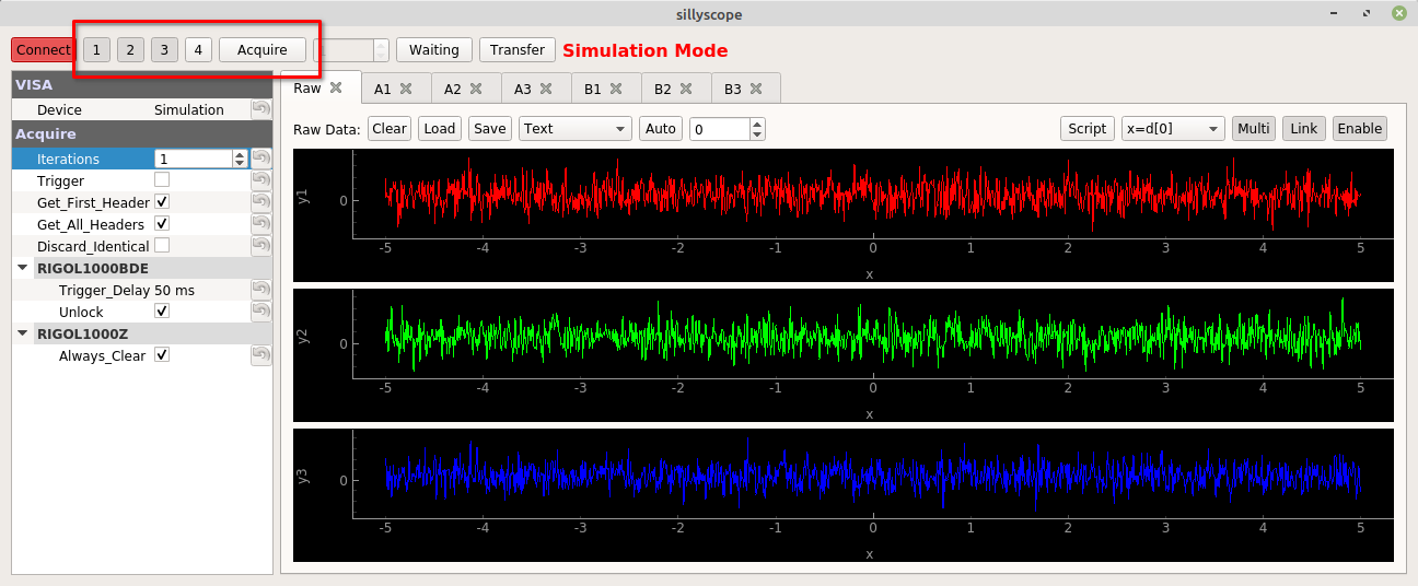
You can change how the program acquires data using the Tree Dictionary s.settings on the left. To learn more about a given setting, select it and hover the mouse over it until a tip pops up.

Finally, sillyscope by default comes with two chains of three Databox Processors, starting with A1 and B1. Every time new data is acquired, it is sent to A1 and B1. If any of these processors have the "Enabled" box checked, the selected processes will be performed in order. For example, if you wish to measure the power spectral densities (pay attention to the Windowing Function!):

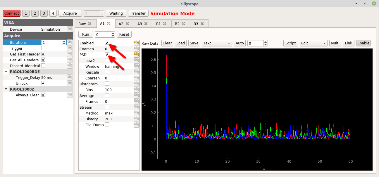
This data is subsequently sent to the next Databox Processor in the chain, so the output of A1 is sent to A2, the output of A2 is sent to A3, and the same happens for the B1, B2, and B3.

Another very helpful functionality is "Autosave", which enables incoming data to be automatically written to an alphabetically time-ordered data file. To enable this feature, press the Auto button on any Databox Plotter:

This should bring up a dialog asking you where to save the file, and what name to give it. In the above, I chose my desktop folder and the file name "pants.txt". Now, every time the plotter receives new data, it will save as a text file to /path/to/desktop/N pants.txt, where N is the number in the box (which then increments). These files will contain all of the settings, and are saved in Spinmob's databox format.

You can read more about how these objects work [here]((https://github.com/Spinmob/spinmob/wiki/6.-Easy-GUI-Generator-(egg)).

Scripting

All actions you can perform with the GUI can be easily scripted. For example, to select a device, connect, select channels, and aquire:

s.settings['VISA/Device'] = 'Simulation'
s.button_connect.click()
s.button_1.set_checked(True)
s.button_2.set_checked(True)
s.button_3.set_checked(True)
s.button_acquire.click()

To enable the A1 processor and coarsen incoming data by 4,

s.A1.settings['Enabled'] = True
s.A1.settings['Coarsen'] = 4

To help you find a given control using autocomplete, all Tree Dictionaries are named settings, all buttons begin with button_, all number boxes will start with number_, all combo boxes begin with combo_ and all Databox Plotters begin with plot_. For example, if you want to find the autosave button on A1's plot, type s.A1.plot.button_autosave. You can then search for set_ and get_ functions to control its state, or click() to simulate a click.