Robot-Motion-Planning-with-Potential-Field-Approach

The Motion Planing in 2D space is done using potential field approach. Special Thanks : Atul Thakur Sir(From IIT Patna)

Problem Statement

1.For an R^2configuration space of size 100m × 100m, define an additive potential field with attractive potential as a combination of conic as well as quadratic potential and repulsive potential determined using Brushfire algorithm. Also determine the gradient of the potential function. Now implement your equations in a Matlab or any other programming language of your choice. Display the gradient vector field using arrows (in Matlab use quiver command). The arrows should be made at (1,1), (2,1)…(100,1), (1,2), (2,2)…(100,2),…(100,100) with the length of each arrow representing the magnitude of the gradient and direction of the arrow the direction of the gradient. You may use the enclosed Matlab implementation of Brushfire algorithm for determining minimum distance function. Note that the obstacles can be loaded via the enclosed image file which can be edited in MS Paint. In your report clearly describe the steps of your entire approach with all the equations. Make a list of the parameters that need to be tuned. Also, show how/whether the vector field changes with variation of tunable parameters and describe.

2.Now, implement a gradient descent approach to calculate a path from any given start point to goal location using the results in (1). Assume that start and goal location will never be specified on any obstacles. Test your algorithm for several start and goal locations. Comment on completeness of the approach you developed.

The Approach taken:

1.The Brushfire algorithm divides the picture into n*n pixels and assigns each pixel a value according to its distance from the wall or obstacle.
  The Attractive Potential Function are made as :

The norm function is used to find the d(q,q_goal) i.e the euclidean distance. The ζ is a tunable parameter and curently its set to 2.

2.The Repulsive Potential Function are made as : 

The Dq parameter is expected to state the distance from the obstacle so it is assigned equal to the value of the world matrix which was made from the brushfire algorithm. And for ∇Dq is the taken from the gradient of the world matrix.

3.The repulsive and additive gradient and potential are then added :

4.Q_start is defined.

Here, p stores all the q points and hence is further used to plot the path.

5.The Quiver function is used the plot the gradient. And along with the path (p) is also plotted.

List of all the tuneable parameters and effect of changing them on the path formed:

1	d*
2	Q*
3	ζ
4	η
5	ϵ
6	α

 

d* : this Parameter is responsible for distance from goal at which the conic potential changes to quadratic potential.The size of the arrow increased as d_star increases. This is because the gradient of conic and quadratic potential are now close.The Path is plotted in blue dots.

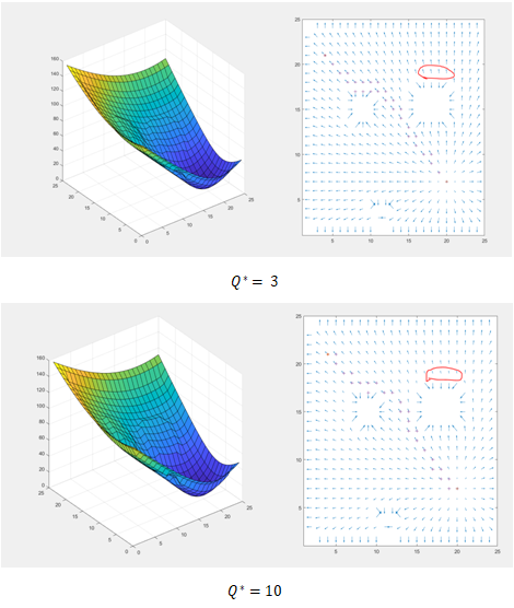
Q* ∶ This parameter can be also called the sphere of influence for the obstacles.The Gradient near the obstacle weakens as Q_star Increases.

ζ∶ This Parameter is responsible for increasing the attractive potential and gradient. The length of the arrows have increased.

η ∶ This Parameter is responsible for increasing the repulsive potential and gradient.The arrows near the obstacle grows as this param increases.

ϵ∶ This parameters control how much far is the from goal,the path should he stop.

α∶ This determines the number of path points.