Reconstruct Image
This module renders (reconstructs) detected localizations from Results table as a probability map. As a result, it generates 32-bit image where each molecule is represented as a 2D Gaussian with integrated intensity of 1. Settings window looks like this:
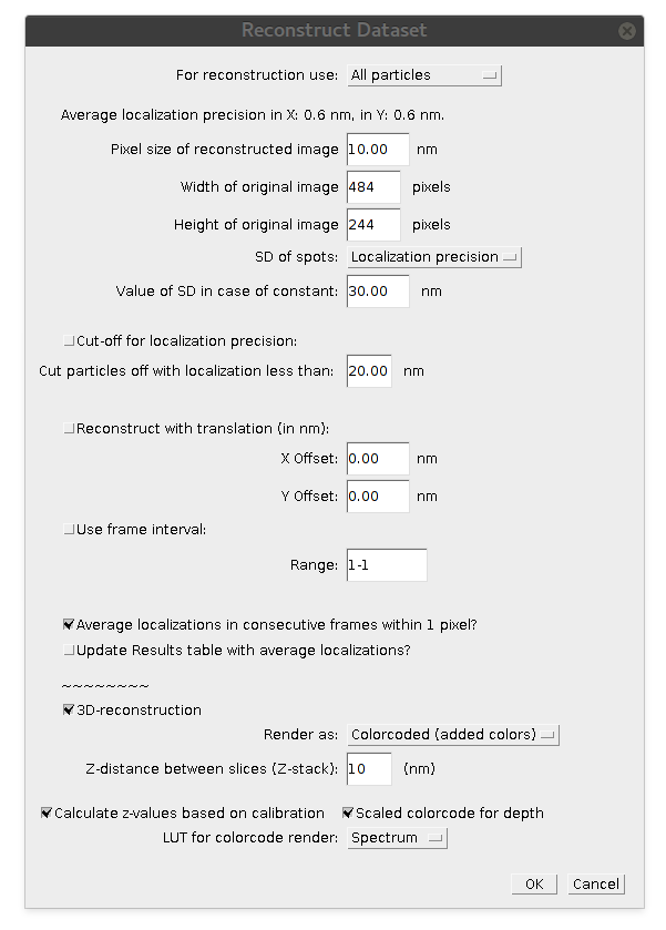
It has following parameters/comments:
Whether to render all particles or only "true positives".
is calculated from Results table and shown here mostly to help with estimation of next parameter.
is in nanometers.
define the area of the reconstructed image in original pixels. Usually they are just dimensions of original stack/image. These values are estimated using max(X_(nm)) and max(Y_nm) columns of Results table and can be overruled to expand/shrink reconstructed area.
Standard deviations in X and Y of rendered Gaussian per spot. In case of Localization precision option the values are picked up from X_loc_error(nm) and Y_loc_error(nm) columns. In case of Constant value renders symmetric Gaussian with SD specified by next parameter.
is in nanometers. It is used to render particles in case of Constant value of previous parameter.
if selected, renders only particles which have localization error in X and Y smaller than the value of the next parameter.
is in nanometers.
shifts all rendered particles by provided values (in nanometers). It is handy for datasets with two-color/channels consecutive acquisitions, if there is drift of microscope's stage. When reconstructing the second channel, final values from Drift Correction table of the first channel can be provided.
if selected, renders only particles from provided range of frames.
option is used to "bin" together multiple frames of photoactivation event for single fluorescent emitter. If selected, the plugin searches for detected positions of particles within one pixel of original image that span some continuous frame interval. Under assumption of sparsity they are treated as localizations of the same molecules. For these events plugin calculates and renders weighted averages of X_(px), Y_(px), X_(nm) and Y_(nm) using corresponding squared values of X_loc_error(nm) and Y_loc_error(nm) as weights.
Rendered values of X_loc_error(nm) and Y_loc_error(nm) are recalculated according to propagation of error principle/formula.
The weighted average procedure happens with mean values and errors of Z_(nm), Amplitude_fit, BGfit, SD_X_(nm), SD_Y_(nm).
Frame_Number and False_positive are simply averaged and rounded.
in case the previous parameter is checked, updates Results table with recalculated values (according to rules above). In addition, for the parameters IntegratedInt, SNR, R2_fit and Iterations_fit just simple average is calculated.
if checked, renders image using particles Z coordinates with options below.
Reconstructs image as a set of Z-slices with distance between them defined by parameter below. At the current moment (August 2016) it does not take into account error in Z localization, i.e. each particle is plotted only once in stack (i.e. it is not rendered as 3D Gaussian).
In this case plugin renders image where Z coordinate is coded by color defined by LUT, color look-up table. How exactly it is done? It picks LUT selected by parameter below and converts each color to HSB space. In short, any color can be represented in RGB space by three numbers, i.e. "intensities" of red, green or blue components. Alternatively, it can be represented by H=hue (kind of "wavelength), S="saturation" and B=brightness (kind of "intensity"). Plugin renders Z coordinate information using hue and saturation, while rendered intensity (localization precision) is coded in brightness value. It is coded in two different ways, more precisely:
In this case if there are two overlapping particles at the same pixel, their intensity will be summed up in B(brightness) channels. Values of H(hue) and S(saturation) will be calculated as weighted averages with intensities as weights. This type of rendering represents bright "transparent" accumulating rendering, making structures with overlapping pixels brighter, in comparison to:
In this case if there are two overlapping particles at the same pixel, H(hue) and S(saturation) values are picked from the particle with highest intensity (so its values becomes final B(brightness)).
in nm, defines (well) distance between slices of rendered Z-stack in case of Render as Z-stack method (see above.
Convenient shortcut, so there is no need to click for and call Calculate Z values. Updated Results table with calculated Z coordinates.
for explanation requires separate page (please click on title).
Color look-up table list loaded from available LUTs at your installation of ImageJ/FIJI.