This repository contains the report and code behind my Neural Computation (VS265 @ UC Berkeley) final project. This project is based off of an essay I wrote titled "Dude, where's my motion perception?"
Elliott Waissbluth, Akshara Methukupalli, Neal Aditya
The motion aftereffect is a well known illusion produced by scrolling motion. After looking away from a scrolling stimulus, an observer will see a world that appears to be breathing and warping against the direction of the former motion. In Weiss et al., a Bayesian framework was introduced to model human motion perception. Their model was interesting because it produced the same errors in velocity estimation that humans make. We seek to expand this model to include a component of temporal feedback from the posterior to the prior through time. We show that our expansion naturally informs the motion aftereffect. This post discusses our implementation, results, and future considerations.
The motion aftereffect is produced when illusory opposite-direction motion is perceived of a still object after the mind has adapted to a particular set of motion vectors. The term "waterfall" describes the conditions by which the effect is created. If you fixate on a waterfall, its downwards motion is perceived and adapted to; look away and you will find any motionless environment to be warping upwards as if the motion of the water was caused by a scrolling background. This illusion is evident when you watch a wheel spin, drive long distances on the highway, or walk along a path. Steven Cholewiak has produced a poignant example of this effect, take a moment to watch it:
https://www.youtube.com/watch?v=jP_jYmbke14
To understand the mechanisms underlying motion aftereffect, it is useful to understand the brain's computational model of motion. An accurate model of visual motion perception was laid forth by Weiss et. al. in their paper Motion Illusions as Optimal Percepts [1]. This model fits a vast library of experimental data, demonstrating great viability to explain the actual underlying computations of the brain. Its distinguishing feature is its tendency to make the same mistakes humans do when evaluating motion data. At its core, the model is powered by an ideal observer. An ideal observer is a statistically informed decision maker based on Bayes' Rule. It acts on what it calculates to be the most probable outcome using whatever information it has. An ideal observer can make errors, but only to the degree that the most probable outcome does not reflect reality. In the case of motion perception, the ideal observer's job is to predict the velocity of an object given visual input from the retina. In more formal terms, the ideal observer selects the argument that maximizes the posterior probability of velocity given image data. This is described by the following equation:

The two components of this equation are the prior, P(v), and likelihood, P(I|v). Most literature dealing with this topic assumes a Gaussian prior centered at zero velocity [1-3]. This is known as the slow speed assumption. It accounts for erroneous components brought about by the likelihood functions which guess unrealistically high velocities given a motion stimulus. The likelihood functions are derived using concepts borrowed from optical flow. To understand the likelihood functions, it is necessary to understand the aperture problem in optical flow. First, we will treat it intuitively. Consider the following figure:

Figure 1: The Aperture Problem
The aperture problem arises when velocity is estimated for a windowed stimulus. In the example in Figure 1, the grate is shown moving in three separate directions. However, viewed through the imposed circular window, all three grates produce the same image sequence. All you can say certainly of the velocity of the grate is the range of possible velocities it might have. The grate might be moving up, left, or somewhere in between; this range of these possible velocities is given by the velocity constraint line [4]. The velocity constraint line can be derived from an image subjected to the brightness constraint, that is, the brightness pattern of a patch of image displaced some distance in the x-direction and some distance
in the y-direction will remain constant. We write this as follows

Taking the first-order Taylor series expansion around , subtracting
from both sides, dividing through by
, then taking the limit as
goes to 0, we have

or in terms of velocity

We can use this to write the equation of the velocity constraint line.


Figure 2: Velocity Constraint Line
The velocity constraint line displayed in Figure 2 is the constraint line that might be derived from Figure 1. You will see in our methods section that the likelihood functions we derive will depend heavily on this equation although it does not present itself in the same form as described above. For our simulations, the image space is sampled through Gaussian windows. These windows give rise to the aperture problem when centered around the edge of a stimulus, as in Figure 1. The resulting probability distributions are centered around the line described by the velocity constraint equation.
It has been hypothesized that the motion aftereffect is directly observable in directionally sensitive neurons in human cortical area M [5]. The directionally sensitive neurons are neurons that activate when stimulated by a visual motion stimulus moving in a particular direction. To elucidate this, consider Figure 3.

Figure 3: MT Neuron Magnetic Resonance Response to Moving Stimuli
Figure 3 shows activation in the MT region of human cortical area over time. In the sections labeled "Exp," subjects watched expanding concentric rings. In the section labeled "Exp/Con," the subjects watched expanding and contracting concentric rings. In sections labeled "Stat," the subjects watched static concentric rings, and reportedly felt a strong motion aftereffect. You can see that the activation does not drop off immediately after the moving stimulus is replaced by a static one. Rather, in leaky-integrator like fashion, the activation slowly drops back to baseline levels. The shaded areas under the curve represent the hypothesized regions of motion aftereffect. In this report, we will demonstrate how this effect naturally arises via a feedback loop from the posterior distribution to the prior distribution.
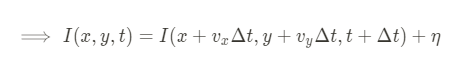
Weiss et. al, like most optical flow models, assume an brightness constraint as seen in the above equations. Under this assumption, an object that moves may change position but not brightness, leaving the intensity function same with a delta change. Formally, this can be written as

and
can written in terms of
and
. Furthermore, there is noise in image perception [2], so we get the following equation
The first order Taylor series expansion of the above equation results in

Substituting in the previous equation:

We can assume a Gaussian noise with standard deviation of , and the Weiss et. al paper assumes that velocity is constant over a Gaussian window w. Therefore, the probability of the intensity function for a particular position can be written as

Unlike Weiss et. al, which assumes a Gaussian prior, since we are assuming the prior probability of the velocity, v, to be the posterior of the previous timestep. This results in the posterior estimation of velocity to be as follows

Figure 4: Feedback model

Weiss et. al furthermore shows two key variables in deriving likelihood functions from an image sequence: contrast and shape. These two variables are important features underlying errors in motion perception. We derived likelihood functions showing the distinction between these two variables to show how the velocity constraint line might change, and to prove that our likelihood functions accurately represented the given image. We used Sobel filters with 5x5 kernels for space derivatives and frame single frame subtraction to approximate time derivatives.

Figure 5: Effect of contrast
Figure 5 shows the likelihood functions derived from high contrast and low contrast images depicting a rhombus moving to the right. To simplify the example, we included samples from two points, though many more were summed to derive a posterior distribution in practice. As expected, the higher contrast image has a tighter likelihood while the lower contrast includes more noise. This matches the findings found in Weiss et. al regarding contrast.

Figure 6: Effect of shape
Similarly, Figure 6 shows the likelihood functions generated by changing the shape of the input, without changing the velocity. A fatter rhombus shows less range in the likelihood of the y-velocity, implying the motion will be more horizontal. This is contrary to the function generated by a skinnier rhombus, which shows more uncertainty in the y-direction.
Although the likelihood functions derived look as expected for single frames, across time we couldn't reproduce reliable likelihood functions. We believe this is due the fact that the space derivatives (Sobel filters) were not flexible enough to accommodate temporal changes. To this end, we created synthetic data to represent the likelihood functions over time.
The above equations were simulated using synthetic data. We used Jessica Hamrick's notes [6] as a starting point to get the data for the initial likelihood function. The following simulations are using the Gaussian prior and a feedback prior
Figure 7 shows the simulation for a Gaussian prior as suggested by the Weiss et. al paper and Figure 8 shows the simulation of a feedback prior. The second and third frames of the images are the likelihoods of the velocities at a given point. After a certain point in time, they become Gaussians centered at 0 emulating a change in motion from a moving object to a stationary object. You can imagine the input image sequence as a rhombus moving right then stopping, as in Figures 5, 6.

Figure 7: Posterior Estimation using Gaussian prior

Figure 8: Posterior Estimation using feedback prior

Figure 9: Posterior estimation of velocity over time
As can be seen from Figure 8, the posterior gradually gravitates to zero. Figure 9 further shows that this change in estimation looks like a leaky integrator. Velocity here is calculated as the distance of the posterior estimation to the origin. This result aligned to the observations from the Tootell et. al's paper on activations in the MT region with a motion aftereffect stimulus (see Figure 2).
The framework we have presented for sensory adaptation to motion is based upon a rapidly changing prior. From the perspective of perception as Bayesian inference, this might seem unintuitive. If a prior is subjected to rapid changes, then why have a prior at all? Surely our perception of the world would be muddled and confusing if our conceived statistical distribution of motion was fluid. Perhaps the best way to account for this is by modeling perception as a cascade of processing stages, a Bayesian estimator built upon hierarchical representations as in [7]. We have presented a slice of this cascade, built upon layers of more invariant representations of motion. From the hierarchical perspective, the prior is a function of the posterior and of the expectation for the world to follow Newtonian physics. We believe this model could be developed to include this system of hierarchy for a more robust representation of motion perception.
In their 2006 paper, Sensory Adaptation within a Bayesian Framework for Perception [13], Stocker and Simoncelli specifically argue against a system in which the prior is modified by adaptation. Their solution to a Bayesian framework for sensory adaptation is an adaptor that increases the signal to noise ratio (SNR) in the vicinity of the parameter value of the adaptor. The motivating principle behind this is sensory repulsion. Consider the motion aftereffect brought upon by a scrolling stimulus moving towards the right. When the motion stops, the illusion produces the sensation of leftward motion, the opposite direction. In our framework, the posterior settles back to zero but only after traversing the velocity space of rightwards motion. If the argument that maximizes the posterior during this settling phase is an estimation that the motionless stimulus is moving right, then why is it that we perceive the stimulus to be moving left? The SNR solution accounts for this, however it relies on the assumption that our perception is directly guided by velocity estimation. If we take velocity estimation as an underlying computational principle to calculate acceleration, with acceleration mapping more directly to our perception, then it is not necessarily true that the attraction of the posterior contradicts the perception of repulsed motion.
Take the simulation we have provided as an example. The motion stimulus drives the posterior distribution to the positive side of velocity space. After the stimulus becomes motionless, the velocity estimation drifts from positive velocity back to the origin. Taking the derivative of the velocity estimation through time, we arrive at acceleration. This drifting phenomena presents itself in acceleration space in the opposite direction of velocity. When velocity goes from positive to zero, acceleration goes from negative to zero. What we perceive when we experience the motion aftereffect is this acceleration field applied to a motionless stimulus. A still picture being pulled in the opposite direction of a previously adapted motion appears to be accelerating in the same direction as that motion coming to a stop. If this is the root cause of the motion aftereffect, then the theory that the prior changes through time does not contradict the repulsion effect noted in psychophysical literature [8-11].
Our model in its current form is not meant to be a rigid computational framework that explains motion perception, it is meant to be a proof of concept demonstrating the viability of a feedback mechanism within the computational framework. In this venture, we believe we have succeeded. There are parts of the model that have room for development and other parts that are counterintuitive. We will acknowledge these shortcomings and discuss potential methods to address them.
The first is the u-shaped trajectory of the velocity estimate once the motion stimulus stops moving. You can see from Figure 8 that the velocity estimation dips below the axis before settling at the origin. This does not necessarily invalidate the solution however a more rigorous review of psychophysical data is required. Intuitively, this
component shouldn't exist. A system more representative of reality would follow a straight path back to the origin. One reason for this behavior is the running sum of the posterior. Without normalization, the posteriors of previous timesteps long forgotten will still be able to influence the path of the posterior distribution as it drifts back to the origin through time.
The second counterintuitive nuance is the shape of the prior once it settles back to zero. It is Gaussian however . This makes sense because the longer you perceive a motionless object, the more sure you are that the object has zero velocity. However, if the prior is a concentrated Gaussian centered at zero then the posterior will not drift effectively to the likelihood functions' estimation of velocity once motion is perceived. This is where a widely spread slow speed assumption Gaussian might be advantageous. Previously we discussed the idea of a hierarchical system influenced by a deeper and more invariant prior. This mechanism could be incorporated into the system to solve this phenomena.
In conclusion, the framework we have proposed expands on a well validated model of motion perception. By introducing a specific mechanism of feedback we have demonstrated an explanation of the phenomena of sensory adaptation specifically in the visual velocity space. The model we implemented is not fully actionable but it is promising for future development. Next steps include improving the derivatives we use to calculate likelihoods, as in [12], and implementing a hierarchical framework.
- Weiss, Y., Simoncelli, E. P., & Adelson, E. H. (2002). Motion illusions as optimal percepts. Nature neuroscience, 5(6), 598-604.
- Stocker, A. A., & Simoncelli, E. P. (2006). Noise characteristics and prior expectations in human visual speed perception. Nature Neuroscience, 9(4), 578–585. https://doi.org/10.1038/nn1669
- Simoncelli, E. P., Adelson, E. H., & Heeger, D. J. (1991). Probability distributions of optical flow. 1991 IEEE Computer Society Conference on Computer Vision and Pattern Recognition Proceedings, 310–315. https://doi.org/10.1109/CVPR.1991.139707
- Horn, B. K., & Schunck, B. G. (1981, November). Determining optical flow. In Techniques and Applications of Image Understanding (Vol. 281, pp. 319-331). International Society for Optics and Photonics.
- Tootell, R., Reppas, J., Dale, A., Look, R., Sereno, M., Malach, R., Brady, T., & Rosen, B. (1995). Visual motion aftereffect in human cortical area MT revealed by functional magnetic resonance imaging. Nature, 375, 139–141. https://doi.org/10.1038/375139a0
- Hamrick, J. (2015, November 9). Demo: Motion Illusions as Optimal Percepts. Retrieved from http://jhamrick.github.io/quals/probabilistic models of perception/2015/11/09/Weiss2002-ipynb.html
- Rao, R. P. (2005). Hierarchical Bayesian Inference in Networks of Spiking Neurons. 1113–1120. http://papers.neurips.cc/paper/2643-hierarchical-bayesian-inference-in-networks-of-spiking-neurons
- P. Thompson. Velocity after-effects: the effects of adaptation to moving stimuli on the perception of subsequently seen moving stimuli. Vision Research, 21:337–345, 1980.
- A.T. Smith. Velocity coding: evidence from perceived velocity shifts. Vision Research, 25(12):1969–1976, 1985.
- P. Schrater and E. Simoncelli. Local velocity representation: evidence from motion adaptation. Vision Research, 38:3899–3912, 1998.
- C.W. Clifford. Perceptual adaptation: motion parallels orientation. Trends in Cognitive Sciences, 6(3):136–143, March 2002.
- Farid, H., & Simoncelli, E. P. (2004). Differentiation of Discrete Multidimensional Signals. IEEE Transactions on Image Processing, 13(4), 496–508. https://doi.org/10.1109/TIP.2004.823819
- Stocker, A. A., & Simoncelli, E. P. (n.d.). Sensory Adaptation within a Bayesian Framework for Perception. 8.