-
Notifications
You must be signed in to change notification settings - Fork 8
Meshing
One of PyFRAP's strength is its flexibility with the experiment geometry. PyFRAP's geometry and meshing functionalities combined with Gmsh allow you to model pretty much any two- and three-dimensional geometry.
Here we explain how to use make use of PyFRAP's geometrical capabilities. Some of PyFRAP's functionalities are integrated in PyFRAP's GUI. Here we explain how to make use of them. PyFRAP's python modules are more powerful. Here we describe how to create and mesh geometries using PyFRAP as a scripted tool.
PyFRAP uses Gmsh, a powerful meshing toolbox, as a backend for geometries and meshing.
PyFRAP's geometries are defined in .geo files that follow Gmsh's notation. PyFRAP can read and write .geo files and load them into python objects for plotting and parameter specification, however, ultimately, the file that specifies the final geometry is the one specified in the .geo file. If you want to learn more about this, please refer to this section.
Even though PyFRAP has its own mesh class, the main property of the mesh are defined in the .geo file that also specifies the geometry. PyFRAP simply reads and writes this file and then executes Gmsh on it. Please refer to this section and the Gmsh manual for further information
PyFRAP's GUI offers multiple ways to specify your experiments geometries. The most simple way it so select one of the preset geometries:
- zebrafishDomeStage: A zebrafish embryo at dome zebra
- cylinder: A cylinder
- cone: A frustum-like geometry
- ball: A sphere.
- custom: A custom geometry
You can select between these presets under Embryo -> Geometry -> Select Geometry. For the first four geometries, PyFRAP comes with already written .geo files and dialogs that allow you to easily edit these geometries via Embryo -> Geometry -> Edit Geometry.
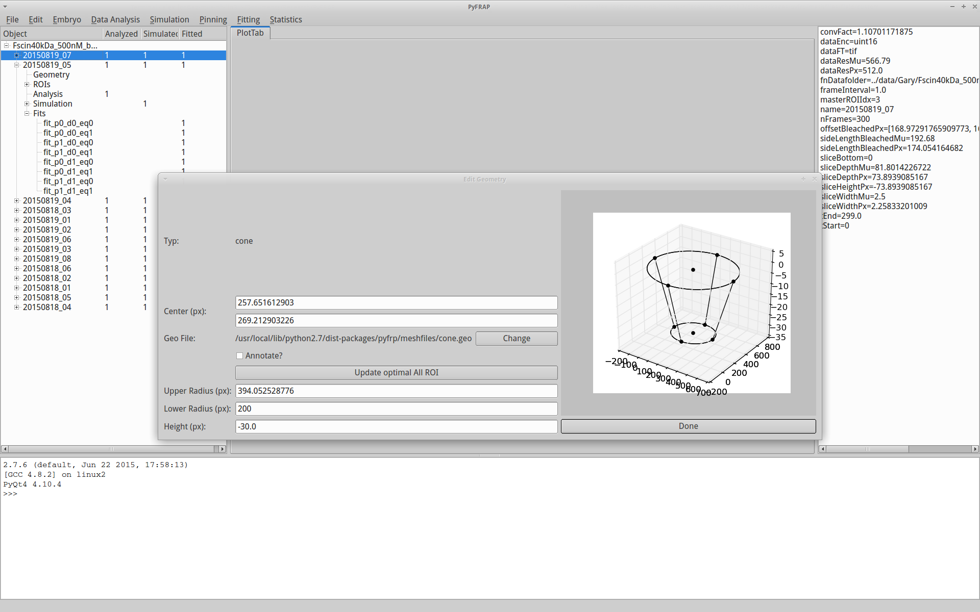
However, you can always access and edit the .geo file directly via Embryo -> Geometry -> Edit Geo File. Please refer to the Gmsh manual for instructions on how geometries are specified in .geo files.
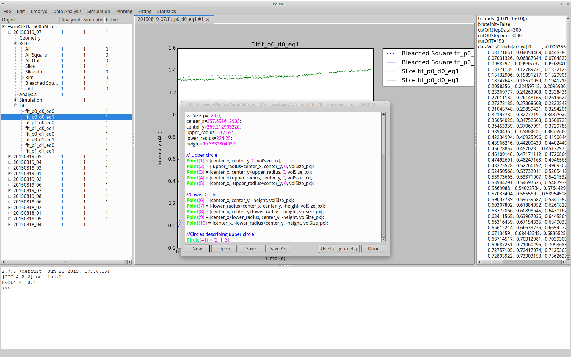
PyFRAP wraps some of Gmsh's meshing capabilities in the GUI. Having a good mesh is crucial for appropiate FRAP analysis with PyFRAP. All meshing options can be accessed in Simulation -> Mesh. The options include:
- Mesh Settings: Basic dialog for meshing, see also FirstSteps.
- Generate Mesh: Calls Gmsh on the current .geo file.
- Refine mesh: Calls Gmsh with the --refine option, refining the mesh by mesh splitting.
- Force mesh density: PyFRAP incrementally refines the mesh until the global mesh density reaches a limit.
- Refine Mesh in ROI: Refines mesh in a given ROI.
- Add boundary layer around ROI: Adds a boundary layer mesh around an ROI.
PyFRAP comes with various meshing methods and is able to make use of most of Gmsh's functionalities. The most important modules for this are
-
pyfrp_gmsh_module: Low-level Gmsh functionalities such as running Gmsh itself. -
pyfrp_gmsh_IO_module: I/O-module for reading/writing .geo/.stl files into PyFRAP. -
pyfrp_gmsh_geometry: PyFRAP classes to describe/build Gmsh geometries, define fields etc.
Most of the functionalities of these modules are integrated in the following subclasses:
-
pyfrp_mesh: Main mesh class. -
pyfrp_ROI: Main ROI class.
Here we describe some examples on how to make use of these functionalities.
The pyfrp_gmsh_geometry.domain class offers a versatile tool to edit and describe geometries that can then be passed to Gmsh for mesh generation.
The domain is a mere canvas that we can draw on, saving all geometrical entities on it, such as
First, lets create a domain:
	from pyfrp.modules import pyfrp_gmsh_geometry
	d = pyfrp_gmsh_geometry.domain()
We can add different geometrical entities, for example a circle:
	volSize=30.

	# Add some vertices
	vcenter=d.addVertex([0,0,0],volSize=volSize)
	v1=d.addVertex([1,0,0],volSize=volSize)
	v2=d.addVertex([0,1,0],volSize=volSize)
	v3=d.addVertex([-1,0,0],volSize=volSize)
	v4=d.addVertex([0,-1,0],volSize=volSize)

	# Add Arcs
	a1=d.addArc(v1,vcenter,v2)
	a2=d.addArc(v2,vcenter,v3)
	a3=d.addArc(v3,vcenter,v4)
	a4=d.addArc(v4,vcenter,v1)
and draw the complete canvas via
d.draw()
to obtain

We can also simply call
d.addCircleByParameters([0,0],1,0,30.)
See also this example.
A simple 3-dimensional geometry is a cylinder. To create a cylinder, simple type
	# Some parameters
	center=[0,0]
	radius=1.
	height=50.
	zOffset=100.
	volSize=30.

	# Add cylinder
	d.addCylinderByParameters(center,radius,zOffset,height,volSize,plane="z",genLoops=True,genSurfaces=True,genVol=True)

	# Draw
	d.draw()

See also this example.
PyFRAP allows you to read in Gmsh .geo files and automatically create a domain object out of it:
	from pyfrp.modules import pyfrp_gmsh_IO_module
	d=pyfrp_gmsh_IO_module.readGeoFile(pathToGeoFile)
Now we can simply add geometrical entities and then write the geometry back into a file:
d.writeToFile(outputFilePath)
Once we've written a domain to a file, we can use it inside our PyFRAP geometry.
emb.geometry.setFnGeo(pathToNewGeometryFile)
Once the geometry is updated, we can use Gmsh to generate a mesh
emb.simulation.mesh.genMesh()
First, we create a geometry with default ROIs:
	# Geometry
	emb.setGeometry2Cone(center,coneUpperRadius,coneLowerRadius,cylinderHeight)

	# Update geometry properties in geo-file
	emb.geometry.updateGeoFile()

	# Create default ROIs
	emb.genDefaultROIs(emb.geometry.getCenter(),imagingRadius,rimFactor=rimFactor,sliceHeightPx=-sliceDepth)

	# Add simulation and mesh
	sim=emb.newSimulation()
We can easily create mesh just describing an ROI and then merge it into the main geometry. We first generate a mesh file for a particular ROI:
fnMeshSlice=emb.getROIByName("Slice").genMeshFile(volSizePx=10)
We then merge the files, which automatically calls Gmsh.
	outPutGeoPath,outPutMshPath=pyfrp_gmsh_IO_module.mergeMeshes([emb.simulation.mesh.fnMesh,fnMeshSlice],outPutGeoPath)
	emb.simulation.mesh.setFnMesh(outPutMshPath)
We can use plotMesh to draw the mesh:
emb.simulation.mesh.plotMesh()
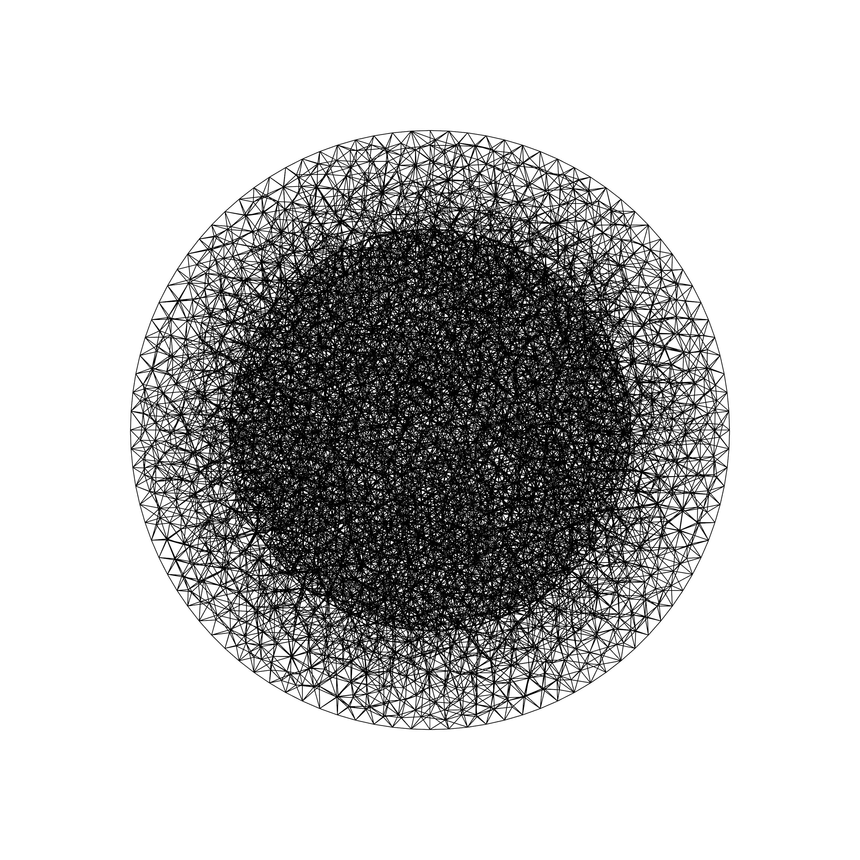
See also this example.
Here we describe how to generate two different boundary layer meshes:
- A boundary layer at the imaging slice.
- A boundary layer around the bleached region
For the first example, we read in the embryos geometry as a domain
	dGeo=emb.geometry.readGeoFile()
	v,a,l,sf=dGeo.addCircleByParameters(center,imagingRadius,-sliceDepth,35.,genSurface=True)
And add a boundary layer field:
	blf=dGeo.addBoundaryLayerField(hfar=35.,hwall_n=10.,hwall_t=10.,thickness=15.,Quads=0.)
	blf.setAsBkgdField()
Luckily, we already created a surface for the added cicle, and thus simply add it to the boundary layer field
sf.addToBoundaryLayer(boundField=blf)
We can write the geometry to a new file, update the location of the .geo file in the embryo's geometry and run gmsh.
	dGeo.writeToFile(fnOut)
	emb.geometry.setFnGeo(fnOut)
	emb.simulation.mesh.genMesh()
We can plot the mesh via
emb.simulation.mesh.plotMesh()
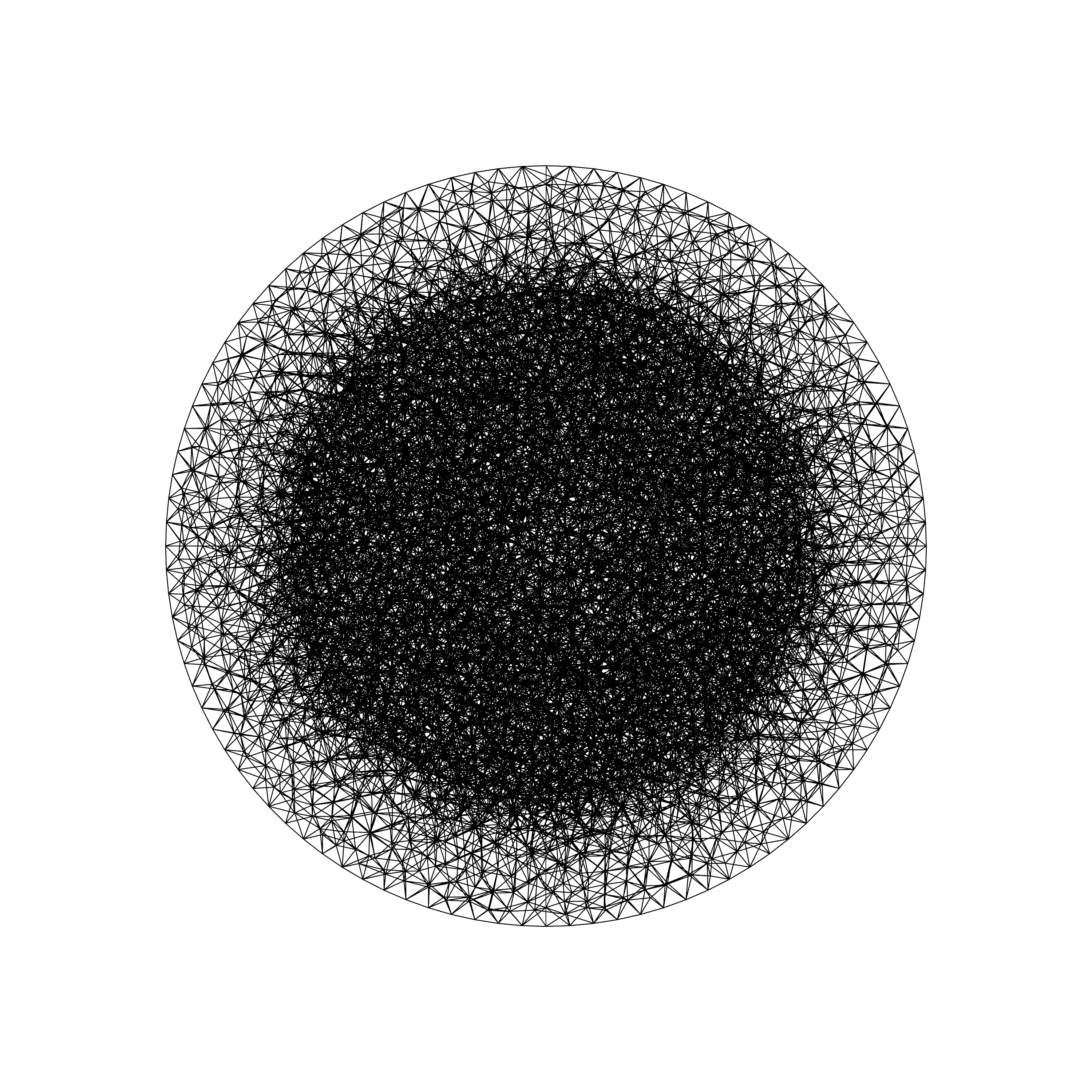
See also this example.
For the second version, we refine the mesh around the bleached region:
	r=emb.getROIByName("All Square")
	sim.mesh.addBoundaryLayerAroundROI(r,fnOut=fnOut,simplify=True,iterations=3,triangIterations=0,
					fixSurfaces=False,debug=False,volSizePx=35.,volSizeLayer=10.,thickness=20.,cleanUp=True,faces=['x','y'])
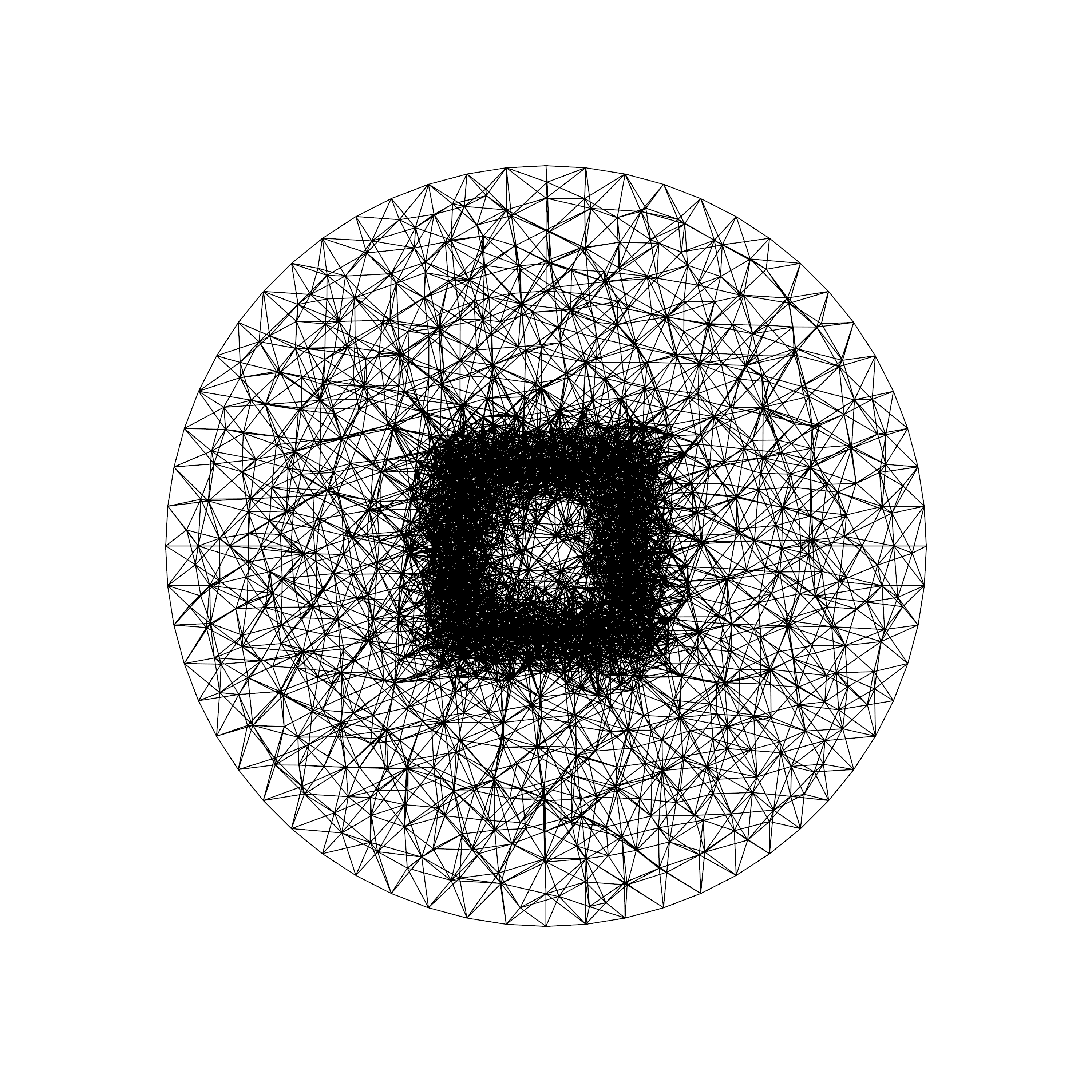
See also this example.