Monte Carlo simulations are a powerful in numerous fields, including operations research, game theory, physics, mathematics, actuarial sciences, finance, among others. It is a technique used to measure risk and uncertainty when making a decision. To put it simple: a Monte Carlo simulation runs an enormous number of statistical experiments with random numbers generated from an underlying distribution based on a given time series. Brownian motion, or random walk, is the main driver for forecasting the future price. On this README file, I will present some results for Bitcoin close price prediction one week from now, including convergence tests for the number of simulations as well as sensitivity analysis for the historical data sample range.
The method consist in obtaining a mean and standard deviation from a given sample data (time series), on this particular case the close price data of Bitcoin from a certain time range. For this article, I will be working with the daily close price.
The Bitcoin historical data was downloaded and saved as .csv file using the Binance API. For this step, it is needed a Binance account and generation of API keys imported from a config.py file with the strings API_KEY and API_SECRET.
import config
from binance.client import Client
from binance.enums import *
import pandas as pd
client = Client(config.API_KEY, config.API_SECRET)
# valid intervals — 1m, 3m, 5m, 15m, 30m, 1h, 2h, 4h, 6h, 8h, 12h, 1d, 3d, 1w, 1M
def print_file(pair, interval, name):
# request historical candle (or klines) data
 bars = client.get_historical_klines(pair, interval, “27 Jun, 2018”, “27 Jun, 2021”)

 # delete unwanted data — just keep date, open, high, low, close
 for line in bars:
 del line[5:]

 # save as CSV file
 df = pd.DataFrame(bars, columns=[‘date’, ‘open’, ‘high’, ‘low’, ‘close’])
 df.set_index(‘date’, inplace=True)
 df.to_csv(name)
print_file(‘BTCUSDT’, ‘1d’, “BTC_1d.csv”)
This step involves essentially reading the .csv file and processing the close price data by obtaining its percentage variation and applying the natural logarithm.
The drift is the direction that rates of returns have had in the past, i.e., the expected return. This parameter is obtained from the mean (μ) and standard deviation (σ) of the given sample.
The volatility is the historical standard deviation multiplied by a random variable (Z), assuming normal distribution.
The expected returns are the given by the natural exponential of the drift plus the volatility.
Observation: since we are dealing with large numbers, there is a high risk of occurring overflow. To deal with this, the natural logarithm of the percentage variation was obtained and then transformed back using the inverse (exponential function) after computing drift and volatility. This mathematical “trick” was used in order to avoid overflow error.
The future price is then obtained by multiplying the price from the past time by the expected return.
This operation is repeated until the desired future date is achieved and then repeated N times to achieve better accuracy. Usually N = 10,000 is a sufficient number of simulations to achieve convergence of probabilities.
From the obtained price data, it is possible to compute probabilities for the future price with a given price range. This was implemented with the function below.
def cdf(array, b, a): # p(r) -> a < r < b
    mean = statistics.mean(array)
    std = statistics.stdev(array)
    p1 = 0.5 * (1 + math.erf((a - mean)/math.sqrt(2 * std**2)))
    p2 = 0.5 * (1 + math.erf((b - mean)/math.sqrt(2 * std**2)))
    return (p2-p1)
Convergence tests were made for different values of N, beginning with N = 10 up to N = 10,000 in order to show convergence of probabilities. The tests were made using Bitcoin daily close price obtained from Binance in the period from 27 of July of 2018 to 27 of July of 2021, which corresponds to a 3 years time series. Forecasting will be made for one week from now. The time series obtained is plotted in the figure below.
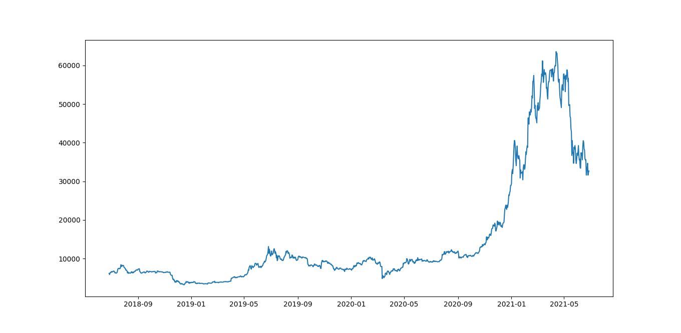
Bitcoin close price time series (daily chart — 3 years span)
Below, is plotted the histogram of the daily expected returns of Bitcoin’s close price, with a black swan event highlighted which probably corresponds to February of 2020 market crash. The drift value obtained from these series was equal to 0.0716%.
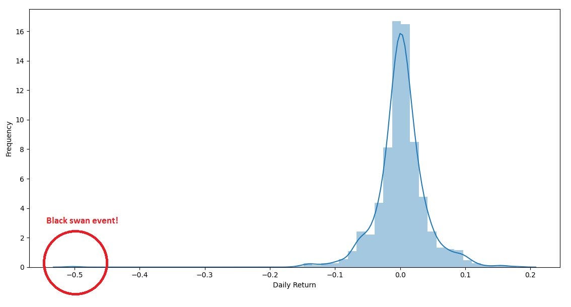
Histogram of Bitcoin’s close price from June of 2018 to the present
In the following figures, it was plotted the predicted time series and the respective histogram of price forecasting one week from now for N = 10, N = 100, N = 1,000 and N = 10,000.
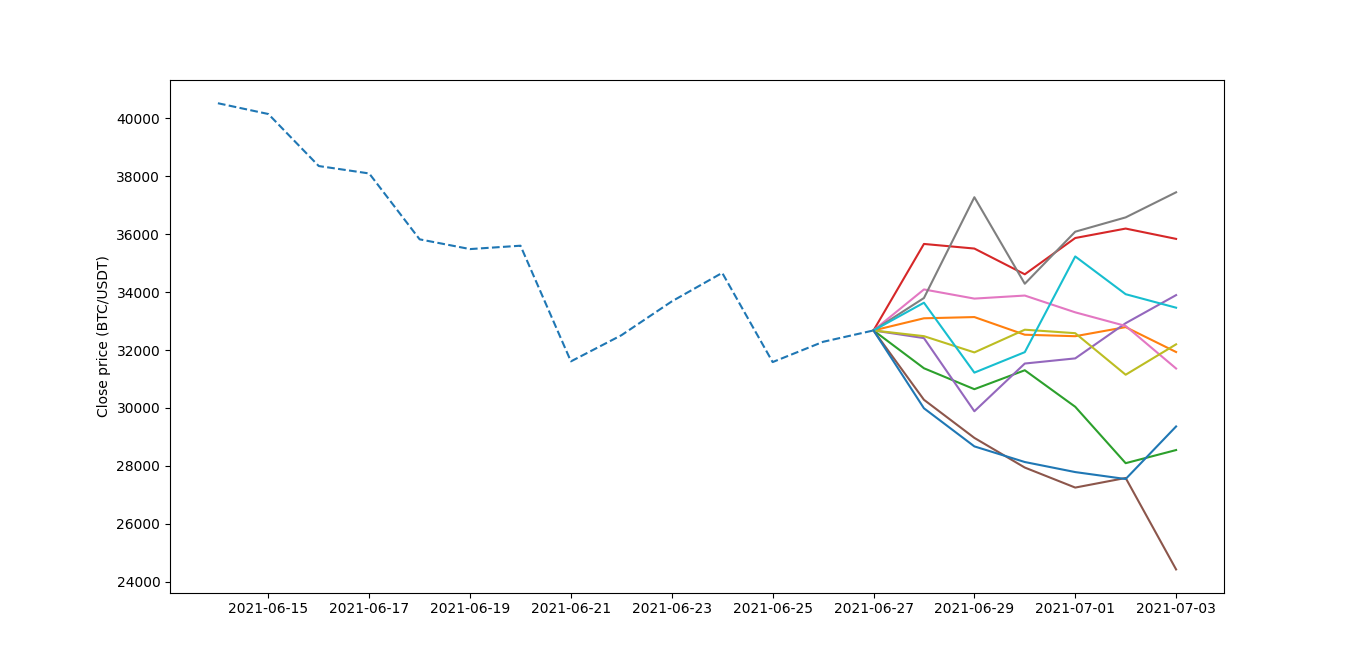
Close price forecasting with N = 10. Each solid line corresponds to one Monte Carlo simulation.

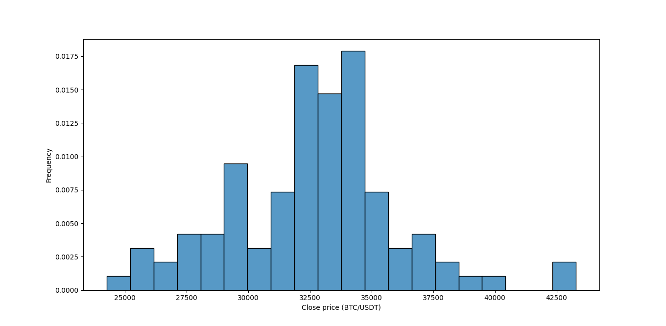
Histogram for one week close price forecasting with N = 10. Very poor results.
Close price forecasting with N = 100. Each solid line corresponds to one Monte Carlo simulation.
Histogram for one week close price forecasting with N = 100. Poor results.
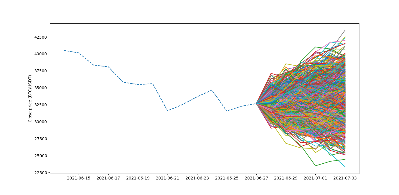
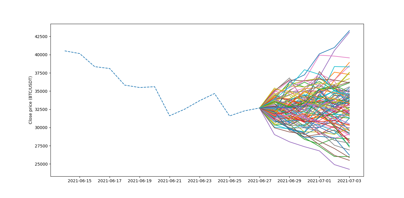
Close price forecasting with N = 1,000. Each solid line corresponds to one Monte Carlo simulation.

Histogram for one week close price forecasting with N = 1,000. Unsatisfactory results.
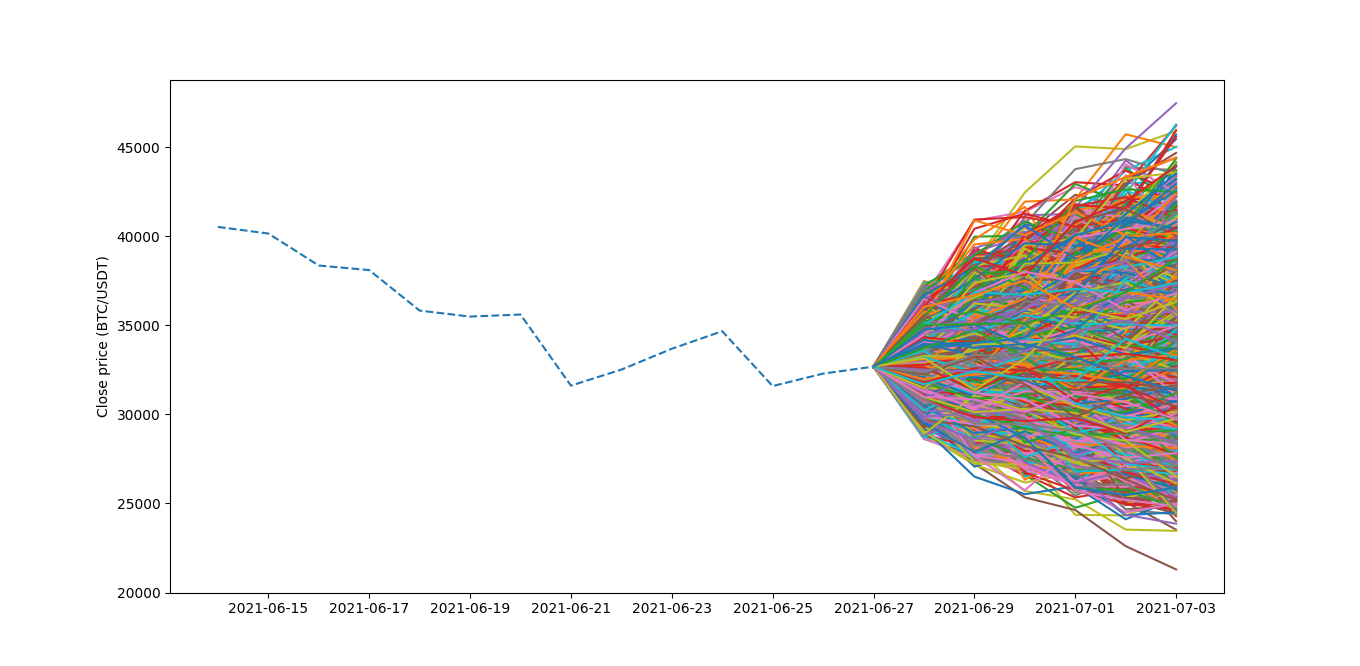
Close price forecasting with N = 10,000. Each solid line corresponds to one Monte Carlo simulation.
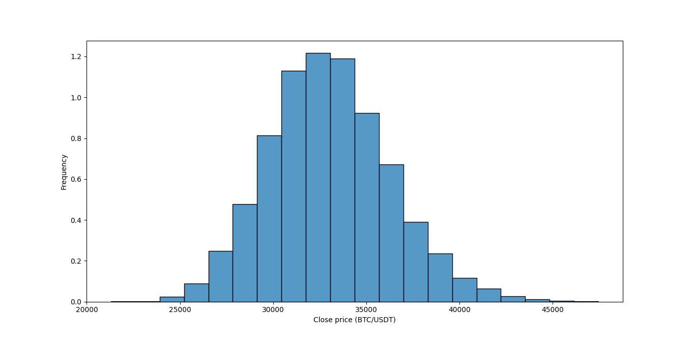
Histogram for one week close price forecasting with N = 10,000. Satisfactory results.
Considering the histograms shown, it can be seen that, as N increased, the histogram converged to a normally distributed curve. This was expected, since in these simulations a normal price variation distribution is assumed. The figure below show the convergence of the probability that the future price of Bitcoin, one week from now, will be between $30,000 and $40,000.
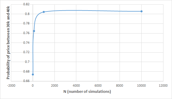
It is observed that convergence is achieved for N = 10,000, as was previously stated, with P($30,000 ≤ close price ≤ $40,000) = 80,57%.
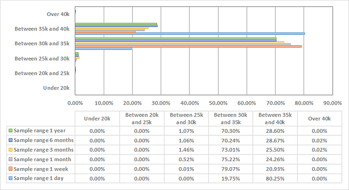
For this section, forecasting of the Bitcoin close price one day from today (09/10/2021) was made through Monte Carlo simulations with N = 10,000 on the hourly chart. Six different sample sizes were analyzed: 1 day, 1 week, 1 month, 3 months, 6 months and one year. The results are shown in the table and chart below.
Bitcoin price range probabilities for 07/10/2021
As seen from the results, one day sample range gives the most outliers compared to the other data sample ranges. A convergence of probabilities is achieved for a sample range of 6 months, with maximum relative difference less than 0,1%.
In this README file, it was presented a demonstration of how a Monte Carlo simulation can be used to forecast future Bitcoin prices and its probability of being in a given price range. Tests were made for different numbers of simulations and convergence was shown to be obtained for N = 10,000. Sensitivity analysis shown that, for a daily forecasting of the Bitcoin price, a sample size of 6 months was shown to yield satisfactory results. It’s important to note that the Monte Carlo simulations assume a normal distribution of returns; however, that is not necessarily the case. While similar, a most precise distribution would be the Cauchy distribution. Nevertheless, for most purposes, the assumption of normal distribution is accurate enough for a large number of trials.