I was recently working with a dataset from an ML Course that had multiple features spanning varying degrees of magnitude, range, and units. This is a significant obstacle as a few machine learning algorithms are highly sensitive to these features.
I’m sure most of you must have faced this issue in your projects or your learning journey. For example, one feature is entirely in kilograms while the other is in grams, another one is liters, and so on. How can we use these features when they vary so vastly in terms of what they’re presenting?
This is where I turned to the concept of feature scaling. It’s a crucial part of the data preprocessing stage but I’ve seen a lot of beginners overlook it (to the detriment of their machine learning model).
Here’s the curious thing about feature scaling – it improves (significantly) the performance of some machine learning algorithms and does not work at all for others. What could be the reason behind this quirk?
Also, what’s the difference between normalization and standardization? These are two of the most commonly used feature scaling techniques in machine learning but a level of ambiguity exists in their understanding. When should you use which technique?
I will answer these questions and more in this article on feature scaling. We will also implement feature scaling in Python to give you a practice understanding of how it works for different machine learning algorithms.
- Why Should we Use Feature Scaling?
- What is Normalization?
- What is Standardization?
- The Big Question – Normalize or Standardize?
- Implementing Feature Scaling in Python
- Normalization using Sklearn
- Standardization using Sklearn
- Applying Feature Scaling to Machine Learning Algorithms
- K-Nearest Neighbours (KNN)
- Support Vector Regressor
- Decision Tree
The first question we need to address – why do we need to scale the variables in our dataset? Some machine learning algorithms are sensitive to feature scaling while others are virtually invariant to it. Let me explain that in more detail.
Machine learning algorithms like linear regression, logistic regression, neural network, etc. that use gradient descent as an optimization technique require data to be scaled. Take a look at the formula for gradient descent below:
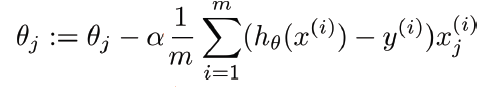
The presence of feature value X in the formula will affect the step size of the gradient descent. The difference in ranges of features will cause different step sizes for each feature. To ensure that the gradient descent moves smoothly towards the minima and that the steps for gradient descent are updated at the same rate for all the features, we scale the data before feeding it to the model.
Having features on a similar scale can help the gradient descent converge more quickly towards the minima.
Distance algorithms like KNN, K-means, and SVM are most affected by the range of features. This is because behind the scenes they are using distances between data points to determine their similarity.
For example, let’s say we have data containing high school CGPA scores of students (ranging from 0 to 5) and their future incomes (in thousands Rupees):
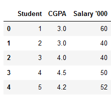
Since both the features have different scales, there is a chance that higher weightage is given to features with higher magnitude. This will impact the performance of the machine learning algorithm and obviously, we do not want our algorithm to be biassed towards one feature.
Therefore, we scale our data before employing a distance based algorithm so that all the features contribute equally to the result.
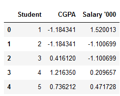
The effect of scaling is conspicuous when we compare the Euclidean distance between data points for students A and B, and between B and C, before and after scaling as shown below:
- Distance AB before scaling
- Distance BC before scaling
- Distance AB after scaling
- Distance BC after scaling
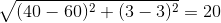


Scaling has brought both the features into the picture and the distances are now more comparable than they were before we applied scaling.
Tree-based algorithms, on the other hand, are fairly insensitive to the scale of the features. Think about it, a decision tree is only splitting a node based on a single feature. The decision tree splits a node on a feature that increases the homogeneity of the node. This split on a feature is not influenced by other features.
So, there is virtually no effect of the remaining features on the split. This is what makes them invariant to the scale of the features!
Normalization is a scaling technique in which values are shifted and rescaled so that they end up ranging between 0 and 1. It is also known as Min-Max scaling.
Here’s the formula for normalization:
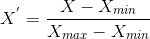
Here, Xmax and Xmin are the maximum and the minimum values of the feature respectively.
- When the value of X is the minimum value in the column, the numerator will be 0, and hence X’ is 0
- On the other hand, when the value of X is the maximum value in the column, the numerator is equal to the denominator and thus the value of X’ is 1
- If the value of X is between the minimum and the maximum value, then the value of X’ is between 0 and 1
Standardization is another scaling technique where the values are centered around the mean with a unit standard deviation. This means that the mean of the attribute becomes zero and the resultant distribution has a unit standard deviation.
Here’s the formula for standardization:

is the mean of the feature values andFeature scaling: Sigmais the standard deviation of the feature values. Note that in this case, the values are not restricted to a particular range.
Now, the big question in your mind must be when should we use normalization and when should we use standardization? Let’s find out!
Normalization vs. standardization is an eternal question among machine learning newcomers. Let me elaborate on the answer in this section.
- Normalization is good to use when you know that the distribution of your data does not follow a Gaussian distribution. This can be useful in algorithms that do not assume any distribution of the data like K-Nearest Neighbors and Neural Networks.
- Standardization, on the other hand, can be helpful in cases where the data follows a Gaussian distribution. However, this does not have to be necessarily true. Also, unlike normalization, standardization does not have a bounding range. So, even if you have outliers in your data, they will not be affected by standardization.
However, at the end of the day, the choice of using normalization or standardization will depend on your problem and the machine learning algorithm you are using. There is no hard and fast rule to tell you when to normalize or standardize your data. You can always start by fitting your model to raw, normalized and standardized data and compare the performance for best results.
It is a good practice to fit the scaler on the training data and then use it to transform the testing data. This would avoid any data leakage during the model testing process. Also, the scaling of target values is generally not required.
Now comes the fun part – putting what we have learned into practice. I will be applying feature scaling to a few machine learning algorithms on the Big Mart dataset I’ve taken the DataHack platform.
I will skip the preprocessing steps since they are out of the scope of this tutorial. But you can find them neatly explained in this article. Those steps will enable you to reach the top 20 percentile on the hackathon leaderboard so that’s worth checking out!
So, let’s first split our data into training and testing sets:
Before moving to the feature scaling part, let’s glance at the details about our data using the pd.describe() method:
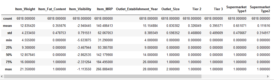
We can see that there is a huge difference in the range of values present in our numerical features: Item_Visibility, Item_Weight, Item_MRP, and Outlet_Establishment_Year. Let’s try and fix that using feature scaling!
Note: You will notice negative values in the Item_Visibility feature because I have taken log-transformation to deal with the skewness in the feature.
Normalization using sklearn To normalize your data, you need to import the MinMaxScalar from the sklearn library and apply it to our dataset. So, let’s do that!
# data normalization with sklearn
from sklearn.preprocessing import MinMaxScaler

# fit scaler on training data
norm = MinMaxScaler().fit(X_train)

# transform training data
X_train_norm = norm.transform(X_train)

# transform testing dataabs
X_test_norm = norm.transform(X_test)
Let’s see how normalization has affected our dataset:
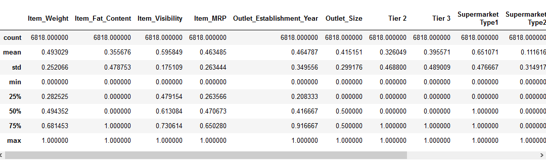
All the features now have a minimum value of 0 and a maximum value of 1. Perfect!
Next, let’s try to standardize our data.
Standardization using sklearn To standardize your data, you need to import the StandardScalar from the sklearn library and apply it to our dataset. Here’s how you can do it:
# data standardization with  sklearn
from sklearn.preprocessing import StandardScaler

# copy of datasets
X_train_stand = X_train.copy()
X_test_stand = X_test.copy()

# numerical features
num_cols = ['Item_Weight','Item_Visibility','Item_MRP','Outlet_Establishment_Year']

# apply standardization on numerical features
for i in num_cols:

    # fit on training data column
    scale = StandardScaler().fit(X_train_stand[[i]])

    # transform the training data column
    X_train_stand[i] = scale.transform(X_train_stand[[i]])

    # transform the testing data column
    X_test_stand[i] = scale.transform(X_test_stand[[i]])
You would have noticed that I only applied standardization to my numerical columns and not the other One-Hot Encoded features. Standardizing the One-Hot encoded features would mean assigning a distribution to categorical features. You don’t want to do that!
But why did I not do the same while normalizing the data? Because One-Hot encoded features are already in the range between 0 to 1. So, normalization would not affect their value.
Right, let’s have a look at how standardization has transformed our data:
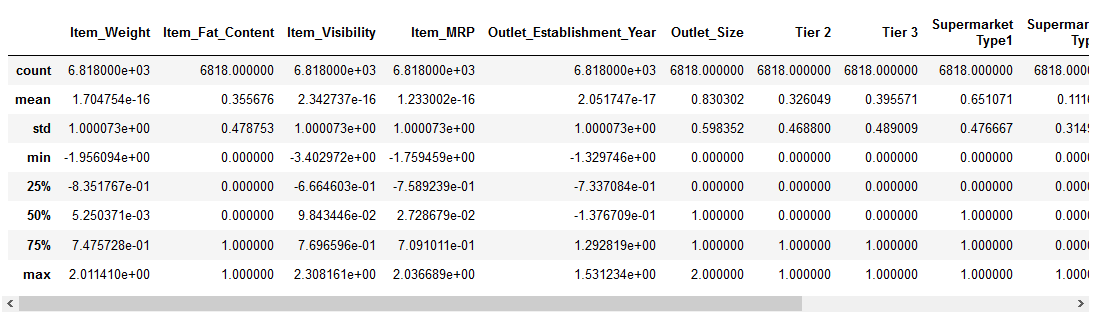
The numerical features are now centered on the mean with a unit standard deviation. Awesome!
Comparing unscaled, normalized and standardized data
It is always great to visualize your data to understand the distribution present. We can see the comparison between our unscaled and scaled data using boxplots.
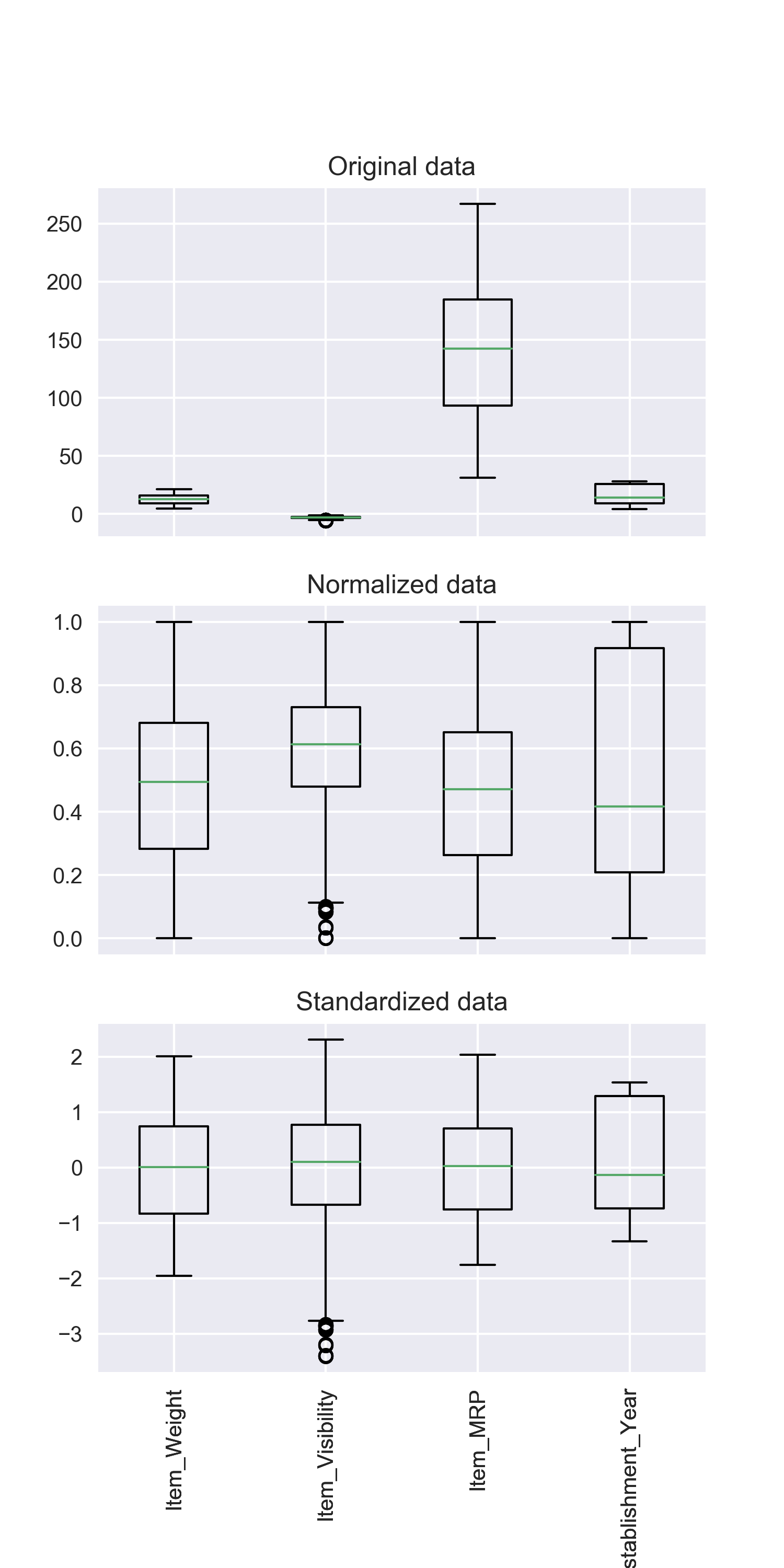
You can notice how scaling the features brings everything into perspective. The features are now more comparable and will have a similar effect on the learning models.
It’s now time to train some machine learning algorithms on our data to compare the effects of different scaling techniques on the performance of the algorithm. I want to see the effect of scaling on three algorithms in particular: K-Nearest Neighbours, Support Vector Regressor, and Decision Tree.
K-Nearest Neighbours
Like we saw before, KNN is a distance-based algorithm that is affected by the range of features. Let’s see how it performs on our data, before and after scaling:
# training a KNN model
from sklearn.neighbors import KNeighborsRegressor
# measuring RMSE score
from sklearn.metrics import mean_squared_error

# knn
knn = KNeighborsRegressor(n_neighbors=7)

rmse = []

# raw, normalized and standardized training and testing data
trainX = [X_train, X_train_norm, X_train_stand]
testX = [X_test, X_test_norm, X_test_stand]

# model fitting and measuring RMSE
for i in range(len(trainX)):

    # fit
    knn.fit(trainX[i],y_train)
    # predict
    pred = knn.predict(testX[i])
    # RMSE
    rmse.append(np.sqrt(mean_squared_error(y_test,pred)))

# visualizing the result
df_knn = pd.DataFrame({'RMSE':rmse},index=['Original','Normalized','Standardized'])
df_knn
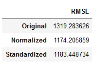
You can see that scaling the features has brought down the RMSE score of our KNN model. Specifically, the normalized data performs a tad bit better than the standardized data.
Note: I am measuring the RMSE here because this competition evaluates the RMSE.
Support Vector Regressor
SVR is another distance-based algorithm. So let’s check out whether it works better with normalization or standardization:
# training an SVR model
from  sklearn.svm import SVR
# measuring RMSE score
from sklearn.metrics import mean_squared_error

# SVR
svr = SVR(kernel='rbf',C=5)

rmse = []

# raw, normalized and standardized training and testing data
trainX = [X_train, X_train_norm, X_train_stand]
testX = [X_test, X_test_norm, X_test_stand]

# model fitting and measuring RMSE
for i in range(len(trainX)):

    # fit
    svr.fit(trainX[i],y_train)
    # predict
    pred = svr.predict(testX[i])
    # RMSE
    rmse.append(np.sqrt(mean_squared_error(y_test,pred)))

# visualizing the result
df_svr = pd.DataFrame({'RMSE':rmse},index=['Original','Normalized','Standardized'])
df_svr
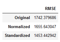
We can see that scaling the features does bring down the RMSE score. And the standardized data has performed better than the normalized data. Why do you think that’s the case?
The sklearn documentation states that SVM, with RBF kernel, assumes that all the features are centered around zero and variance is of the same order. This is because a feature with a variance greater than that of others prevents the estimator from learning from all the features. Great!
Decision Tree
We already know that a Decision tree is invariant to feature scaling. But I wanted to show a practical example of how it performs on the data:
# training a Decision Tree model
from sklearn.tree import DecisionTreeRegressor
# measuring RMSE score
from sklearn.metrics import mean_squared_error

# Decision tree
dt = DecisionTreeRegressor(max_depth=10,random_state=27)

rmse = []

# raw, normalized and standardized training and testing data
trainX = [X_train,X_train_norm,X_train_stand]
testX = [X_test,X_test_norm,X_test_stand]

# model fitting and measuring RMSE
for i in range(len(trainX)):

    # fit
    dt.fit(trainX[i],y_train)
    # predict
    pred = dt.predict(testX[i])
    # RMSE
    rmse.append(np.sqrt(mean_squared_error(y_test,pred)))

# visualizing the result
df_dt = pd.DataFrame({'RMSE':rmse},index=['Original','Normalized','Standardized'])
df_dt
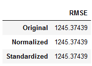
You can see that the RMSE score has not moved an inch on scaling the features. So rest assured when you are using tree-based algorithms on your data!
End Notes
This tutorial covered the relevance of using feature scaling on your data and how normalization and standardization have varying effects on the working of machine learning algorithms
Keep in mind that there is no correct answer to when to use normalization over standardization and vice-versa. It all depends on your data and the algorithm you are using.