Example 13 : Silo
This example performs a three-dimensional discrete element method simulation of filling and evacuation of a silo [1]. We use a stopper at the bottom of the silo to pack the particles. After filling the silo, we remove the stopper and let the particles to leave the hopper.
Total simulation time is equal to 40 s, while time-step, log frequency and output frequency are set equal to 0.00001, 1000 and 1000, respectively:
# --------------------------------------------------
# Simulation and IO Control
#---------------------------------------------------
subsection simulation control
  set time step                 			 = 1e-5
  set time end       					 = 40
  set log frequency				         = 1000
  set output frequency            			 = 1000
end
We use checkpoints to write the simulation information every second. If the simulation breaks or we need to pause it, we could use the checkpoint to resume the simulation instead of restarting it.
#---------------------------------------------------
# Restart
#---------------------------------------------------
subsection restart
	set checkpoint       				 = true
	set filename      				 = sliding_restart
	set frequency					 = 100000
end
In the model parameters section, particle-particle and particle-wall broad and fine search frequencies are defined. We also define the particle contact search size (neighborhood threshold), contact forces and integration methods. The contact detection method is dynamic, and it needs dynamic contact search size coefficient (a safety factor for dynamic contact search). Load-balancing redistributes the computational load on the processors every 2 s, in case of parallel simulations to decrease simulation time.
# --------------------------------------------------
# Model parameters
#---------------------------------------------------
subsection model parameters
  set contact detection method 		   		 = dynamic
  set dynamic contact search size coefficient	 	 = 0.8
  set load balance method				 = frequent
  set load balance frequency				 = 200000
  set neighborhood threshold				 = 1.3
  set particle particle contact force method             = pp_nonlinear
  set particle wall contact force method                 = pw_nonlinear
  set integration method				 = velocity_verlet
end
In the physical properties section, the physical properties of particles and walls, including diameter and density of particles, Young's modulus, Poisson's ratios, restitution coefficients, friction and rolling frictions of particle and wall are chosen. The gravitational acceleration is also set in this section. Diameter of particles in this example is 5.833 mm. The experiments [1] used non-spherical barley grains. We used spherical particles with the same volume. Total number of particles in this example is 132300.
#---------------------------------------------------
# Physical Properties
#---------------------------------------------------
subsection physical properties
    set gx            		 			= 0.0
    set gy            		 			= 0.0
    set gz            		 			= -9.81
    set number of particle types	                = 1
    	subsection particle type 0
		set size distribution type		= uniform
    		set diameter            	 	= 0.005833
		set number				= 132300
    		set density particles            	= 600
    		set young modulus particles         	= 5000000
    		set poisson ratio particles          	= 0.5
    		set restitution coefficient particles	= 0.7
    		set friction coefficient particles      = 0.5
    		set rolling friction particles         	= 0.01
	end
    set young modulus wall            			= 5000000
    set poisson ratio wall            			= 0.5
    set restitution coefficient wall           		= 0.7
    set friction coefficient wall         		= 0.5
    set rolling friction wall         	      	  	= 0.01
end
Next, we define the insertion properties, which are insertion method, inserted number of particles at each insertion step, insertion frequency, insertion domain and other information regarding the initial positions of particles inside the insertion domain.
#---------------------------------------------------
# Insertion Info
#---------------------------------------------------
subsection insertion info
    set insertion method				= non_uniform
    set inserted number of particles at each time step  = 20000
    set insertion frequency            		 	= 20000
    set insertion box minimum x            	 	= -0.37
    set insertion box minimum y            	        = -0.042
    set insertion box minimum z            	        = 0.9
    set insertion box maximum x            	        = 0.37
    set insertion box maximum y           	 	= 0.007
    set insertion box maximum z            	        = 1.09
    set insertion distance threshold			= 1.5
    set insertion random number range			= 0.1
    set insertion random number seed			= 19
end
We use a mesh file for this simulation. Gmsh [2] generates this mesh file.
#---------------------------------------------------
# Mesh
#---------------------------------------------------
subsection mesh
	set type = gmsh
	set file name = ./silo.msh
end
We define a stopper to pack the particles during filling. The stopper locates at z=0 m. We remove the stopper at t=4 s to start silo evacuation.
#---------------------------------------------------
# Floating Walls
#---------------------------------------------------
subsection floating walls
    set number of floating walls	                = 1
    	subsection wall 0
		subsection point on wall
			set x				= 0
			set y				= 0
			set z				= 0
		end
		subsection normal vector
			set nx				= 0
			set ny				= 0
			set nz				= 1
		end
		set start time				= 0
		set end time				= 4
    	end
end
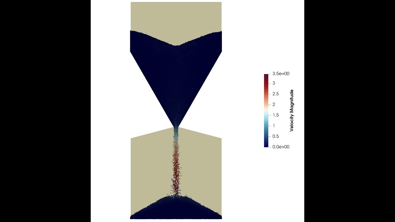
dem_3d solver simulates this example. A snapshot of the silo during evacuation of particles:

Watch the animation of this simulation:
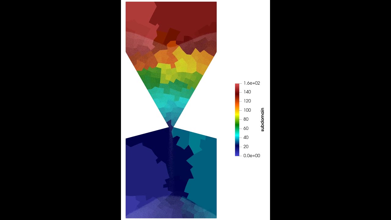
Watch the dynamic distribution of domains in a simulation on 160 processes. As particles move inside the simulation domain, load-balancing equalizes the load on the processes.
[1] Golshan, S., Esgandari, B., Zarghami, R., Blais, B. and Saleh, K., 2020. Experimental and DEM studies of velocity profiles and residence time distribution of non-spherical particles in silos. Powder Technology, 373, pp.510-521.
[2] Geuzaine, C. and Remacle, J.F., 2009. Gmsh: A 3‐D finite element mesh generator with built‐in pre‐and post‐processing facilities. International journal for numerical methods in engineering, 79(11), pp.1309-1331.