Tutorial

Basic tutorial

Description	Picture
To run VizBin double click the VizBin-dist.jar icon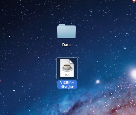
Upon your first run, VizBin will initialize the settings only once. This window will not appear in future executions of VizBin.
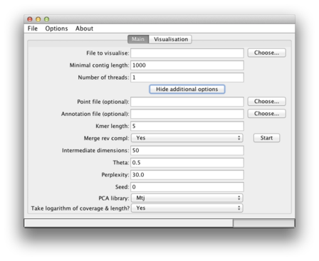
This is how the main window looks like.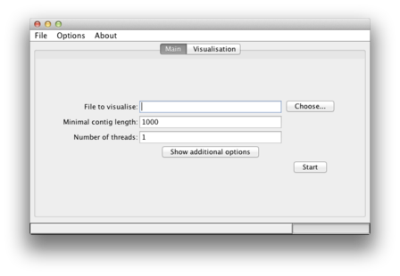
To specify the input sequences in fasta format, click on the "Choose" button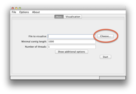
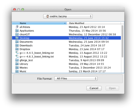
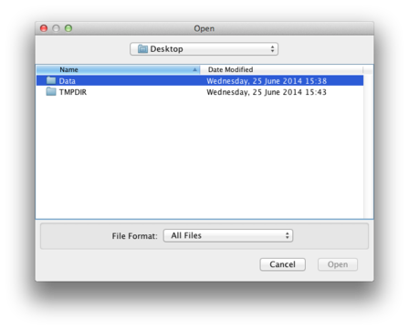
Navigate to the directory containing your input sequences in fasta format. Here, we have them in Desktop/Data/
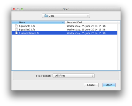
Choose your file of interest, here EssentialGenes.fa
The path to your file of interest should now appear in the "File to visualize" box.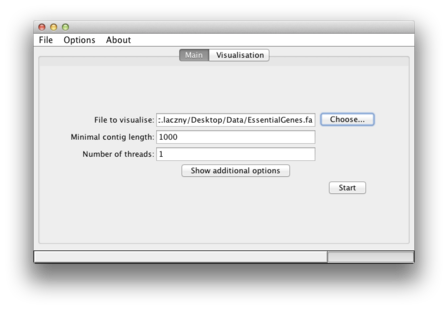
To start, simply click on the "Start" button.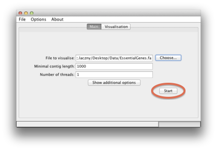
Upon successful termination, a scatterplot will appear in which you will be able to select your clusters of interest. Please also have a look at the general note below.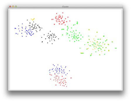
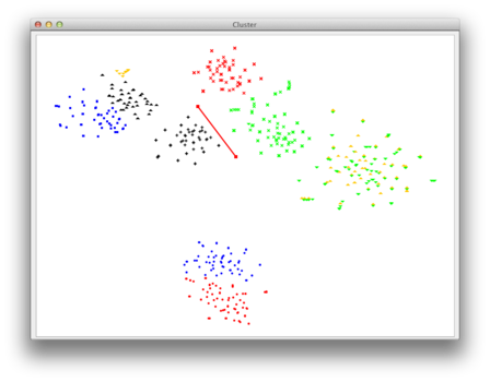
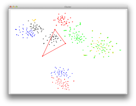
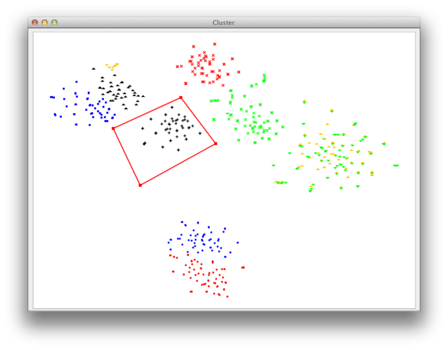
Now you can choose your group of points for which you want the corresponding sequences to be exported to a seperate fasta file. Simply use the left mouse-click to create a polygonal selection. All sequences corresponding to the points inside of this polygon will be exported.
Clicking the right mouse button (anywhere within the visualization) will open a menu where you can choose to export your selection. A confirmation window will apear.
Press "yes" to continue exporting. Press "No" if you want to continue with your selection. Press "Cancel" if you want to start with a fresh polygonal selection without saving the current selection.
Finally, choose the destination for your to-be-exported sequences and give the file a name, here EssentialGenes_Polygon01.fa.

A general note

We tried hard such that VizBin would produce identical between different platforms. However, due to various reasons (e.g., different optimizations done by the different (cross-)compilers, different numerical precision) the resulting 2D scatterplots might look slightly different but should be comparable qualitatively. In other words, it can happen that running VizBin on a Linux-machine or on a Windows-machine with the same input fasta file will give you slightly different visualizations. However, the difference should be only in the relative position but not overall shape of the individual clusters. Hence, a particular cluster might not be at the same position on both machines but the clusters should be readily separated from other clusters and thus should be intuitively selectable with the polygon.

Advanced options

Here we explain what the additional options (hidden by default) allow you to do. After clicking on "Show additional options", you will see different fields which can be modified:

Option name	Explanation
Point file (optional)	After computation of the 2D coordinates, this data is available in the points.txt file in the temporary directory (see your log-file). Specifying this file here makes VizBin create a visualization based on this previously computed data. A basic check is integrated to verify if the number of sequences specified in the "File to visualise" matches the number of points in points.txt. However, it is up to you to make sure you are indeed using the same sequences that were used in the initial creation of the chosen points.txt file. A future version of VizBin will integrate a convenient way of saving a session including the sequences, computed 2D coordinates etc.
Annotation file (optional)	This file allows you to provide additional information that will the be displayed by size, color, and/or opaqueness of individual points. The format of the file is CSV, i.e., the columns must be separated by a comma. The first line of the file must contain information on what information you provide in which column and only the following types are currently supported and have to be specified exactly as listed: label, length, isMarker, coverage, and gc. You may provide them in any order, e.g., coverage,length,label,isMarker, however, coverage and gc are mutually exclusive. Besides this header line, the following lines must match the order of the contigs in the fasta file and contain the information per column corresponding to the type of that column in the header. Accordingly, the first anntation line corresponds to the first sequence, the second annotation line to the second sequence and so on. You can find an example annotation file in example dataset AMFJ01.
Kmer length	This specifies the length of the k mer that is used to compute the genomic signature. We found k = 5 to work best. This value can be decreased or increased but bare in mind that the number of possible k mers grows exponentially: 4^5 for k = 4, 4^6 for k = 6 etc. We have not yet tested the behavior of the application for larger k than 5.
Merge rev compl	This "collapses" k-mers and their reverse complements to mitigate strand bias.
PCA columns	This represents the number of dimensions (principal components) that are kept when running the initial PCA. The default of 50 is suggested by the original BH-SNE publication.
Theta	More details on different values of "Theta" can be found in the original BH-SNE publication.
Perplexity	More details on different values of "Perplexity" can be found in the original BH-SNE publication. As a general note, should you have a small number of sequences, e.g., below 100, then you should decrease the perplexity value. Think of it as the expected number of neighbors. This might help you to choose a reasonable smaller value. Start maybe by decreasing it slowly from the default value. Since you have few sequences, the computation should be fast.
Seed	BH-SNE is solving a non-convex optimization problem. Thus, the solver can end up in a local optimum which must not necessarily be a global optimum. Setting this value to something different than the default of "0" allows you to see if a different initialization leads to a markedly improved result. We found that the results are generally robust with respect to different initializations. Please note that the 2D scatterplots will be different in shape but should be qualitatively comparable. Make sure to remember this value and adust it if you want to reproduce results obtained on the same machine.
PCA library	We integrated two libraries for computing the PCA. The default Mtj is more efficient, in particular on large datasets This is, among others, due to some optimization we integrated. It should work on all platforms. For legacy reasons, we also provide the PCA version of EJML.
Take logarithm of coverage & length?	This option allows you to transform your coverage & length values using the natural logarithm (i.e., at the base e. This is enabled by default but should you provide your own transformation of the coverage & length values, simply set it to Noand VizBin will use the values you specified without any transformation. This option is only effective if you provide an annotation file containing this information, s.a. Annotation file above.