These are all the notes I've taken while studying for system design interivews. The top resources I've used are:
- Designing Data Intensive Applications, by Martin Kleppmann
- jordanhasnolife's System Design 2.0 Youtube channel
- ByteByteGo's System Design Fundamentals Youtube Channel
- Donne Martin's System Design Primer on Github
But I also reference other resources and articles as well, which I link in an "Additional Reading" section at the end of each topic module.
I'm currently working on turning these notes into an interactive study tool called System Design Daily. You can check that out here
Feel free to open a pull request if there are any inaccuracies in the content
In this section, we'll take a look at some formats for storing data, examining the pros and cons of each. This will include topics like relational data models, column compression, and SQL v.s NoSQL databases. We'll also look at some frameworks for encoding the data to be sent over the network, like JSON, XML, Protobuf, and Avro
Relational data, or the relational model for representing data, is an intuitive, straightforward way of representing data in tables. Each table in our relational database only represents one type of data model. Relationships between tables are represented using foriegn IDs, which map two rows in two tables together. For example:
We have a companies table representing our companies
| Id | Company |
|---|---|
| 1 | Company A |
| 2 | Company B |
| 3 | Company C |
We have an cities table representing cities
| Id | City Name |
|---|---|
| 1 | San Francisco |
| 2 | Seattle |
| 3 | New York |
A company offices table could be the result of joining the two tables, which tells us which companies have offices in which cities.
| CompanyId | CityId |
|---|---|
| 1 | 1 |
| 1 | 3 |
| 2 | 2 |
| 2 | 3 |
| 3 | 1 |
Relational data is sometimes referred to as "normalized" data. A relational database is a type of database that stores this data, and typically uses SQL (Structured Query Langage) for querying and updating.
As mentioned before, SQL is a programming language for storing and processing information in a relational database. It's declarative, meaning we specify the expected result and core logic without directing the program's control flow. Imperative, on the other hand, directs the control flow of the program. In other words, in declarative programming "you say what you want", whereas in imperative programming you "say how to get what you want".
Declarative languages are good for database operations because they abstract away the underlying database implementation, enabling the system to make performance improvements without breaking queries. Furthermore, declarative languages lend themselves well to parallel execution, since they only specify the pattern of results and not the method used to determine them. Unlike with imperative code, the order of operations doesn't matter.
In practice, SQL statements can be executed in a specific way to maximize cache hits and ensure good performance. Many database systems have query optimizers which do these reorderings automatically behind the scenes.
Relational database tables in a single node might not be stored near each other on disk (poor data locality). That means trying to do the join across two tables could be slow due to random I/O on disk. In a distributed system, these tables might not even live on the same database node due to partitioning (which we'll get into later). This would require us to make multiple network requests to different places, among other problems related to data consistency.
Another issue that arises with relational data stems from the fact that many programming languages are object-oriented, meaning applications interact with data classes and objects. Relational data, with tables and rows, might not necessarily translate well - this issue is called Object-relational Impedance Mismatch. The most common way to mitigate this is through the use of Object-Relational Mappers (ORMs), which do exactly as their name implies - they translate objects to relational data and vice versa.
Nonrelational data uses a denormalized data model. For example, we could represent the same "company offices" relation above as a dictionary:
{
  "Company A": ["San Francisco", "New York"],
  "Company B": ["Seattle", "New York"],
  "Company C": ["San Francisco"]
}
Now, we have better data locality since we don't have to query a company table and cities table separately to get the joined company offices results, everything we need is contained right there in the dictionary.
However, this means that we have repeated data keys ("San Francisco", and "New York"). Not only does this mean we need to store more data, this also means modifying our data could potentially be more complicated. If we wanted to remove "New York" from our list of cities, we'd need to update our data in multiple places.
In general, we want to use non-relational data when all of our data is disjoint. For example if we have posts on Facebook, they're typically not related to each other, and can be represented in a denormalized fashion. However, if we need to represent data types that might be related, such as which authors wrote certain books, we might be better served going with a relational database.
Row-oriented storage has data for a single row stored together, which is basically like your regular relational database table. For example, the Employees table stored as employees.txt:
| Name | Company | |
|---|---|---|
| Alice | alice@email.com | |
| Bob | bob@email.com | Amazon |
| Charlie | charlie@email.com |
Column oriented storage stores a bunch of column values together. So rather than having the Name, Email, and Company all in the same file, we split out each column into its own file and just store the value of that column for each row. For example we'd have a companies.txt, emails.txt, and names.txt:
| Company |
|---|
| Amazon |
| ... |
(You can extrapolate the above to apply to emails and names as well)
Using column oriented storage gives us several advantages:
- We can do faster analytical queries over all or a large set of the values in our data for just a single column
- Column compression can also be performed to minimize the amount of data being stored (see below)
- Since we have less data in this scenario, we can even store it in memory or CPU cache for even faster reads/writes.
Imagine we have the following table:
| Name | Followers |
|---|---|
| Alice | 3 |
| Bob | 3 |
| Charlie | 1 |
| David | 1 |
| Edward | 2 |
| Frank | 5 |
| Gordon | 4 |
If we have column oriented storage, we can easily compress the "Followers" file using bitmap encoding:
| Followers | Bitmap Encoding |
|---|---|
| 1 | 0011000 |
| 2 | 0000100 |
| 3 | 1100000 |
| 4 | 0000001 |
| 5 | 0000010 |
The way this works is: We see that Charlie and David (3rd and 4th in our table) both have only 1 Follower, so for the 1 Follower row, we set the 3rd and 4th bits in our bitmap going left to right and leave the rest as zeroes. (Hence, 0011000 in the "1 Follower" row)
We can compress this bitmap further by using a run length encoding:
| Followers | Bitmap Encoding | Run-Length Encoding |
|---|---|---|
| 1 | 0011000 | 223 |
| 2 | 0000100 | 412 |
| 3 | 1100000 | 25 |
| 4 | 0000001 | 61 |
| 5 | 0000010 | 511 |
The run length stores the bitmap encoding as a sequence of the count of consecutive zeroes and count of consecutive ones. For example, "0011000" is 2 consecutive 0's, 2 consecutive 1's and 3 consecutive 0's, resulting in "223".
Performing column compression enables us to:
- Send less data over the network
- Potentially keep more data stored in memory or CPU cache if the dataset is small enough
There are a few downsides to column oriented storage:
- Every column must have the same sort order.
- Writes for a single row need to go to different places on disk (This can be improved via an in-memory LSM tree/SSTable set-up since that preserves the sort order of columns).
- Apache Parquet is an open-source column-oriented data file format designed for efficient storage and retrieval. It provides some nice features like:
- Metadata containing minimum, maximum, sum, or average values for each data file chunk, which enables us to efficiently perform queries
- Efficient data compression and encoding schemes
- Amazon Redshift is a column-oriented managed data warehouse solution from AWS
- Apache Druid is a column-oriented, open source, real-time analytics database
In this section, we'll take a look at some data serialization formats and their advantages and disadvantages
CSV stands for "Comma Separated Values". Data is this format is stored as rows of values delimited by commas. CSV is typically easy parse and read, but it doesn't guarantee type safety on the column values or even guarantee values to be present at all:
For example:
rownum,name,age,company
1,alice,24,albertsons
2,bob,twenty-five,amazon
3,charlie,22
Notice that "bob" has an string-type "age" value, and "charlie" is missing a "company" value entirely.
JSON, or Javascript Object Notation, is a plain text, human-readable format that represents data as nested key-value pairs and arrays. JSON is widely used on the web (pretty much every language has some kind of JSON-parsing library).
Example of a JSON object
{
    "userName": "Mantis Toboggan",
    "age": 80,
    "interests": ["partying", "business"],
    "photoAlbum": [
        {
            "url": "images/01.jpg",
            "width": 200,
            "height": 200
        },
        {
            "url": "images/02.jpg",
            "width": 200,
            "height": 200
        }
    ]
}
JSON isn't the most space-efficient due to repeated keys or duplicated data (the "url", "width", and "height" tags above, for example), and also doesn't have type safety guarantees.
XML, or eXtensible Markup Language, is another plain-text, human-readable format that structures data as a series of nested tags. It's similar to HTML, except instead of using a set of predefined tags (h1, p, body), it uses custom tags defined by the author.
Example of an XML object:
<friendsList>
    <friend>
        <name>Mantis</name>
        <age>80</age>
    </friend>
    <friend>
        <name>Mac</name>
        <age>47</age>
    </friend>
</friendsList>
Like JSON, XML doesn't guarantee type saftey and isn't super memory efficient since we have repeated tags around all our data.
Protocol Buffers and Thrift are binary encoding libraries developed by Google and Facebook respectively for serializing data. Here, we define a schema for data and assign each data key a numerical tag, which grants smaller data size since we just use these tags instead of strings.
Example of a Protocol Buffers schema definition:
message Person {
    required string user_name       = 1;
    optional int64  favorite_number = 2;
    repeated string interests       = 3;
}
The schemas provide type safety since they require us to specify what type everything is, as well as nice documentation for other engineers working with our system. However, writing out the schemas require manual dev effort, and the resulting encodings are also not as human-readable.
Apache Avro is a data serialization format that was first developed for Hadoop (which you can read more about here). It uses JSON for defining data schemas and serializes to binary. Data in Avro is typed AND named, and columns can be compressed to save memory. It can also be read by most languages (with Java being the most widely used), though inspecting an Avro document manually requires special Avro tools since the data is serialized in binary.
Example of an Avro JSON schema:
{
    "type": "record",
    "name": "userInfo",
    "fields": [
        {
            "name": "username",
            "type": "string",
            "default": "NONE"
        },
        {
            "name": "favoriteNumber",
            "type": "int",
            "default": -1
        }
    ]
}
One nifty thing Avro can do for us is generate database schemas on the fly based off column names and reconcile different reader / writer schemas. For example, if we have two different schemas being published by two different servers writing to our database, Avro can automatically handle those by filling in missing values between the two schemas with default values.
An example scenario:
Server A's Schema
{
    "type": "record",
    "name": "userInfo",
    "fields": [
        {
            "name": "username",
            "type": "string",
            "default": "NONE"
        },
        {
            "name": "favoriteNumber",
            "type": "int",
            "default": -1
        }
    ]
}
Server B's Schema
{
    "type": "record",
    "name": "userInfo",
    "fields": [
        {
            "name": "username",
            "type": "string",
            "default": "NONE"
        },
        {
            "name": "age",
            "type": "int",
            "default": -1
        }
    ]
}
If we try to read data published by Server A using Server B's schema, Avro will automatically ignore the "favoriteNumber" type. Since that data won't contain an "age" column, it will automatically use our default value of -1.
- Designing Data-Intensive Applications, Chapter 3, "Storage and Retrieval", section 3: "Column-Oriented Storage"
- Designing Data-Intensive Applications, Chapter 4, "Encoding and Evolution", section 1: "Formats for Encoding Data"
- jordanhasnolife System Design 2.0 Playlist:
- Stephane Maarek "Avro Introduction"
A database index is a data structure that allows you to efficiently search for specific records in your database. Below are a few database index types to know.
In a hash index, we pass each database key into a hash function and store the value at a memory address corresponding to the hash. This gives us extremely optimized reads and writes, as hash tables provide constant time lookup and storage
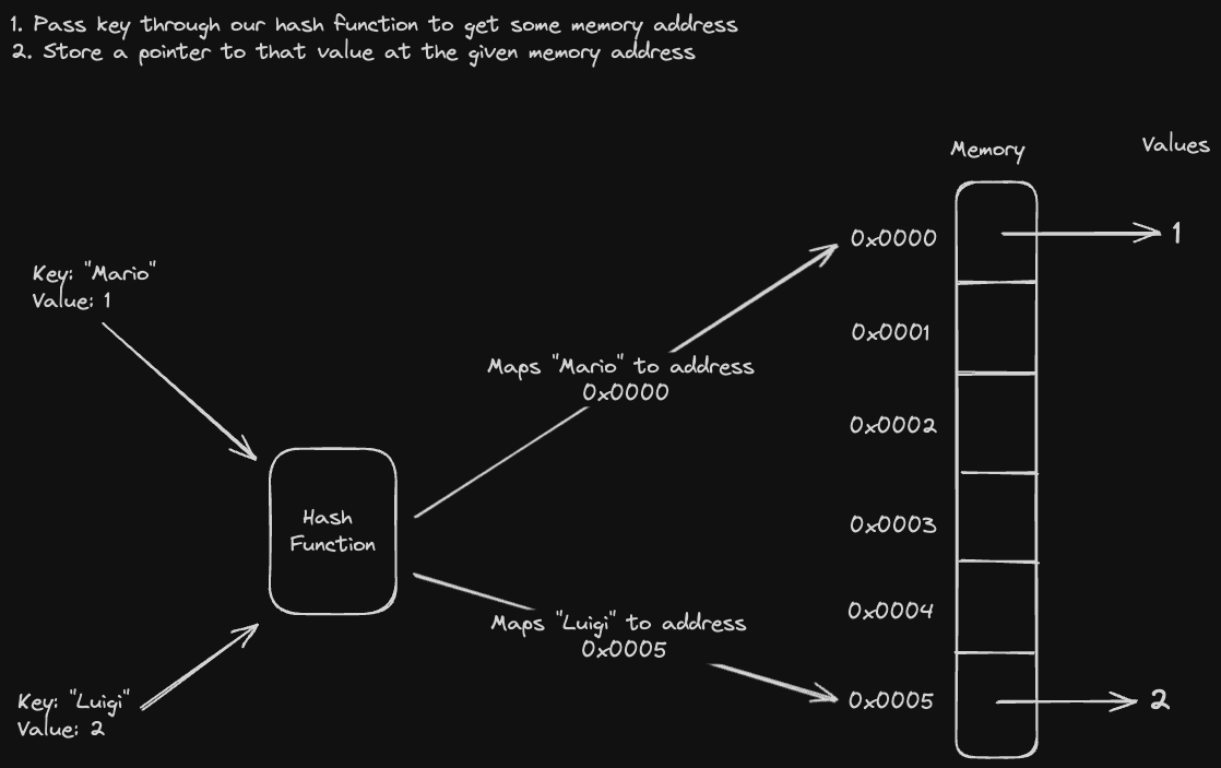
However, hash indexes are limited to small datasets since the hash of the key might not fit within the memory address space. Though you could implement a hash index on disk, it's not efficient to perform random I/O. Furthermore, they're not particularly good for range queries, since the keys aren't sorted. Grabbing all values across "A" and "B", for example, would require us to either check every possible key (which is infeasible), or iterate through all of the keys in our hashmap (which is slow).
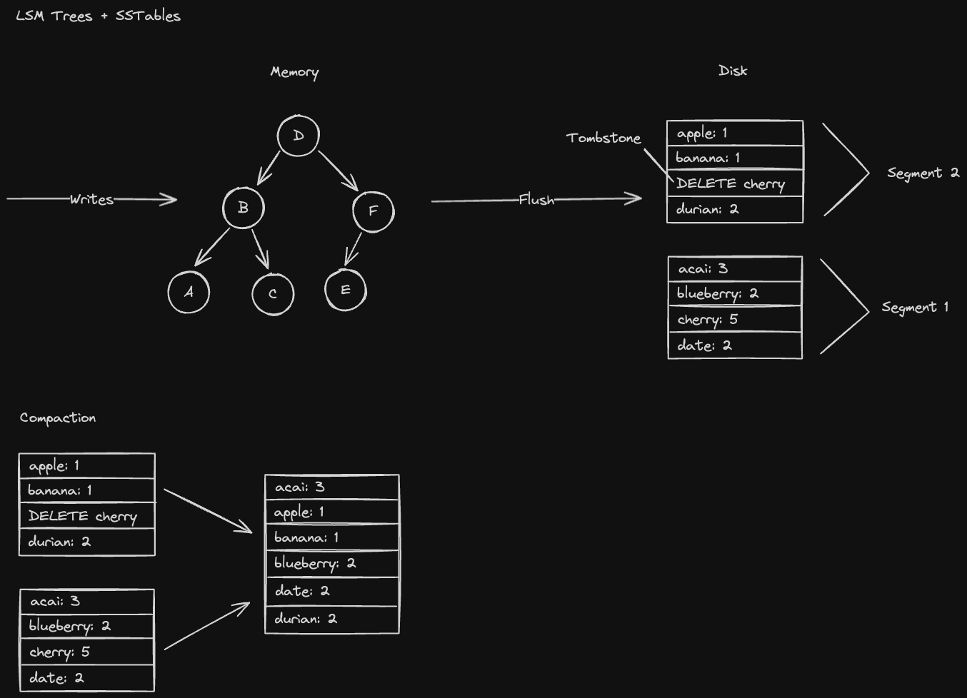
LSM trees are tree data structures used in write-optimized databases. "LSM" stands for “Log Structured Merge Tree” and "SSTable" stands for “Sorted String Table”.
In general, they're optimized for write throughput since we’re writing to a data structure in memory (fast) before writing to disk (slow). In addition, the sorted nature of SSTables allow us to write sequentially to disk which is much faster than writing randomly.
As mentioned before, LSM Trees are auto-balancing binary search trees (e.g. Red-Black trees) that we insert database keys into. Once it gets to be a certain size, we flush the LSM tree to disk as an SSTable. We do a tree traversal to preserve the sorted ordering of keys
Every time we do this SSTable serialization, we create a brand new SSTable which might store new values for keys that exist in previous SSTables. We never delete values from SSTables, instead we store a marker indicating that the value was deleted called a "tombstone"
- This means that reading might be slow since we’d need to scan every SSTable if the key doesn’t exist in our current LSM Tree
- However, we can merge SSTables together in a background process called SSTable compaction (a process similar to the "merge" operation in the mergesort algorithm) reducing the number of SSTables we need to search through.
Here's an example for how this process works:
A write-ahead log (WAL) is just a log of all the write operations we are doing whenever we insert keys into the tree. We maintain a write-ahead log on disk to maintain the durability of the LSM tree.
- Durability means "survivability in the event of failures". For example, if somebody trips on a power cord and wipes our LSM tree in memory, we can recover using the operations we recorded in our WAL
The following systems all use LSM Trees (sometimes referred to as a memtable) and SSTables
- Apache Cassandra, an open source NoSQL database
- Apache HBase, the "Hadoop database", an open source, non-relational big data store
- LevelDB, an open source key-value storage library developed by Google
- RocksDB, a high performance embedded key-value store, which is actually a fork of LevelDB developed and maintained by Facebook
Note: All of the above systems store data as LSM Trees and SSTables rather than index data in that way.
B Tree indexes are database indexes that utilize a self-balancing N-ary search tree known as a B tree, and are the most widely used type of index. Unlike LSM trees and SSTables, B tree indexes are stored mostly on disk.
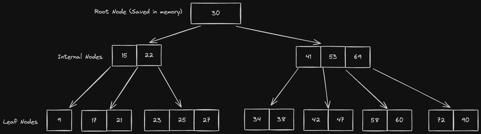
B Trees have a special property in that each node contains a range of keys in sorted order, and there is a lower and upper bound on the number of keys and children that a node may have:
- These bounds are usually determined by the size of a page on disk
- Inserting into a node might trigger a cascading series of splits to preserve the balance of the binary tree, which may incur some CPU penalties. However, the advantages we get in terms of read efficiency are typically worth these downsides
Reading from B Trees is generally fast due to the high branching factor (large number of children at each node). To be more specific, since an internal B tree node can have more than just 2 children, the logarithmic time complexity will have a higher base than 2
B+ Trees are similar to B Trees, except:
- Whereas B Trees can store data at the interior node level, B+ Trees only store data at the leaf node level
- Leaf nodes are linked together (every leaf node has a reference to the next leaf node sequentially).
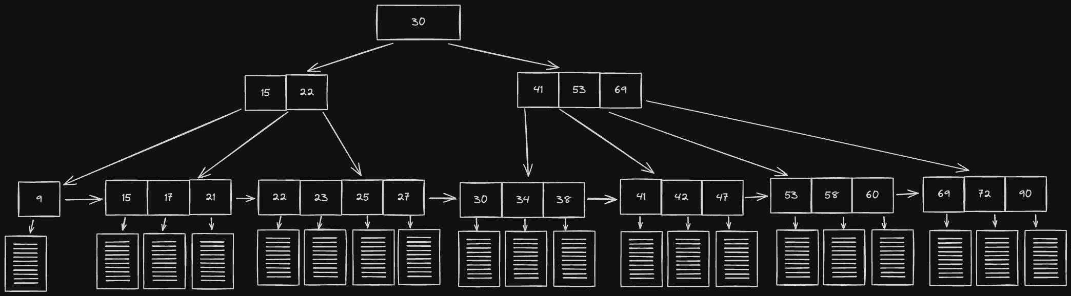
The key advantage offered by this setup is that a full scan of all objects in a tree requires just one linear pass through all leaf nodes, as opposed to having to do a full tree traversal. The disadvantage is that since only leaf nodes contain data, accessing data might take longer since you have to go deeper in the tree
B Trees are used by most relational databases, for example:
- InnoDB, the storage engine of MySQL, an open source relational DBMS
- Microsoft SQL Server, a proprietary DBMS developed and maintained by Microsoft
- PostgreSQL, another open source relational DBMS
However, some non-relational databases use them as well, such as
- MongoDB, a document oriented NoSQL database
- Oracle NoSQL, a NoSQL, distributed key-value database from Oracle
- Designing Data-Intensive Applications, Chapter 3: "Storage and Retrieval", section 1: "Data Structures that Power Your Database"
- jordanhasnolife System Design 2.0 Playlist:
- ByteByteGo System Design Video Series: "The Secret Sauce Behind No SQL"
ACID is an acronym descripting a set of properties referring to database transactions. Transactions are a single unit of work that access and possibly modifies the contents of a database. ACID stands for Atomicity, Consistency, Isolation, and Durability
- Atomicity: Every transaction either completely succeeds or completely fails (no half-measures)
- Consistency: The data in the database is always in a "correct" state. If there are database invariants, the data must respect those
- Isolation: Every concurrent database operation must produce the same result as if the operations were run in sequential order on a single thread
- Durability: The data can be recovered in the event of failure
Read committed isolation is the idea that a database query only sees data committed to before the query began and never sees uncommitted data or changes committed by concurrent transactions. This ensures that our database is protected against dirty writes and dirty reads
- Dirty writes: When two concurrent writes conflict with each other and cause inconsistency in the database
- Solution is row-level locking - if I’m writing to this row, it’s locked and you can’t do anything to it until I release that lock
- Dirty read: Reading uncommitted data: data is modified by a pending write, which causes inconsistency when reading (for example in the event that the write fails)
In practice, Read Committed isolation can be enforced as an isolation level setting for all transactions processed by your DBMS. It provides an intermediate level of isolation when compared to other isolation levels:
- Read Uncommitted (Low): Allows reading uncommitted data (dirty reads)
- Read Committed (Intermediate): Allows only reading of committed data. However, reading a value twice may result in different values (non-repeatable)
- Read Repeatable (High): Allows only reading of commited data and only by a single transaction at a time using exclusive read locks.
- Serializable (Highest): Serializable execution pretty much guantees that transactions appear to be executing in serial order and, by definition, provide the highest isolation level
Consider the following example. We have the following list doctors and patients:
Dr. Toboggan: 2
Dr. Phil: 3
Dr. Oz: 2
Dr. Doom: 1
Dr. Patel: 2
Let's assume we have a query that just goes down the list one at a time. We have an invariant over the table that there are a total of 10 patients at ALL times.
However, let's now assume that before we begin reading Dr. Oz, one patient transfers from Dr. Oz to Dr. Toboggan.
So now, we have the following:
Dr. Toboggan: 2 (now updated to 3)
Dr. Phil: 3
Dr. Oz: 1 < READ
Dr. Doom: 1
Dr. Patel: 2
But now there's a problem. We've already read that Dr. Toboggan only had 2 patients. However, due to this write happening in the middle of our read, we now see that a patient has gone missing. This state, in which our read is over an inconsistent state of the database, is called read skew.
Snapshot isolation is a guarantee that all transactions will see a consistent snapshot, or state, of the database. This addresses the example that we saw above.
Snapshot isolation also guarantees that a write will only successfully commit if it does not conflict with any concurrent updates made since that snapshot.
Snapshots similar to a write-ahead log, in that they display the last committed values in a database for a given point in time. So in our example above, our read query (let's assume it occurs at time T1) would see a snapshot of the database prior to the write, when the patient was transferered.
[T1] Dr. Toboggan: 2
[T1] Dr. Phil: 3
[T1] Dr. Oz: 2
[T1] Dr. Doom: 1
[T1] Dr. Patel: 2
Every time we complete a transaction, we store the resulting value for a given key alongside a timestamp. We hold on to previous values for a given key so that at any given time we can see what the last written value was.
Write Skew
Write skew occurs when writing a value to the database with an invariant over all the data, another concurrent write of which the original write is unaware may put the database in an inconsistent state
Consider this example where we have a table of doctors with columns "name" and "status", which could be either ACTIVE or INACTIVE:
| Name | Status |
|---|---|
| Dr. Toboggan | Active |
| Dr. Oz | Active |
| Dr. Phil | Inactive |
We then have an invariant (rule) that at least 1 doctor needs to be active at all times. If two transactions concurrently try to set "Dr. Oz" and "Dr. Toboggan" to "INACTIVE", they'll both read that there are 2 "ACTIVE" doctors allowing each to set its respective doctor to "INACTIVE", violating the invariant.
In other words, the end result of BOTH writes violate the invariant. This means row-level locking doesn’t work since the invariant is applied over ALL data instead of just one row. What we need is a predicate lock over ALL rows affected by the invariant.
Phantom Writes
A phantom write can occur when two concurrent writes try to both add the same new row. No locks can be grabbed since the row doesn’t even exist yet, resulting in duplicate rows being added to the table.
For example, imagine we have a meeting room booking application, where rooms can be booked from 11AM to 2PM for 1 hour time slots. Users add a new entry whenever they book a room for a time slot:
| Room | Time Slot |
|---|---|
| Room 1 | 1PM - 2PM |
| Room 2 | 11AM - 12PM |
Now if two people try to book Room 2 for 1PM to 2PM at the same time, for example, they could potentially both add duplicate rows to the table. That would not be good.
One way to mitigate this is to pre-populate the database with all rows that could potentially exist. This approach is known as "materializing conflicts". For example:
| Room | Time Slot | Status |
|---|---|---|
| Room 1 | 11AM - 12PM | RESERVED |
| Room 1 | 12PM - 1PM | RESERVED |
| Room 1 | 1PM - 2PM | FREE |
| Room 2 | 11AM - 12PM | FREE |
| Room 2 | 12PM - 1PM | RESERVED |
| Room 2 | 1PM - 2PM | RESERVED |
Now we can use row level locking to ensure only one user is able to book the room for a given time slot!
Of course, this approach isn't feasible for all use-cases. Some storage engines like InnoDB provide "next-key locking" to check for duplicate rows. However, if your storage engine doesn't allow this, you may have to enforce serializable isolation, preventing concurrent transactions from occurring altogether.
Actual Serial Execution forgoes concurrent transactions entirely. Instead, we just process transactions in serialized fashion on a single core and try to optimize processing on that single core as much as possible. Some of these optimizations could include:
- Writing everything in memory instead of on disk, enabling us to use things like hash and self-balancing tree indexes. This means we can’t store as much data
- Use stored procedures - save SQL functions in the database and only accept the parameters of the function to cut down on the amount of data sent over the network
- Stored procedures are somewhat of an antipattern in the real world nowadays since they can lead to inflexible and hard-to-maintain code
The following systems use Actual Serial Execution to maintain isolation:
- VoltDB, an in-memory database
- Redis, an open source in-memory store used as a database, cache or message broker
- Datomic, a distributed database based on the logical query language Datalog
Two Phase Locking is a concurrency control method for enforcing transaction isolation. As the name suggests, it's based on the idea that we have 2 kinds of locks over our database rows and we should apply and release them in phases.
The two distinct phases for applying and removing locks are:
- Expanding phase: Locks are acquired and no locks are released.
- Shrinking phase: Locks are released and no locks are acquired.
The two types of locks we use are:
- Read locks (shared lock) for whenever we’re reading data. That prevents writes from happening to the row, but still allows other reads
- Write locks (exclusive lock) for whenever we’re writing data. This prevents both reads and other writes
Deadlocks
Deadlocks occur when two writes are dependent on each other and neither can release their locks until the other does so in turn (a circular dependency). Let's imagine the following scenario:
Two users each maintain a shopping cart:
Alice: [Apples, Oranges]
Bob: [Milk, Eggs]
Let's imagine this is some kind of "social shopping" app where each user can see each other's cart. If Alice reads from Bob's cart and decides she wants to add Bob's items to her own, she will execute a transaction with the following steps.
- Grab a read lock on Bob's cart (to read his items)
- Grab a read lock on Alice's cart (since we need to read in her items before we can update)
- Grab a write lock on Alice's cart to do the update
However, what if Bob also does the same thing?
- Grab a read lock on Alice's cart
- Grab a read lock on Bob's cart
- Gragb a write lock on Bob's cart to do the update
Now, we have a problem. Neither Alice nor Bob can perform step 3 and grab write locks on their own carts to update them, since write locks are exclusive. So in order for Alice to grab her write lock, she will need Bob to release his read lock on her cart. But Bob can't do that until his write completes.
The only way forward would be for this to be detected by the system, and one transaction would be forced to abort.
Phantom writes
As discussed earlier, this is when we try to acquire locks on rows don't yet exist. Let's imagine we have a table of doctor's appointments, and each doctor can only see one patient at each particular time slot
| DoctorName | PatientName | Time |
|---|---|---|
| Dr. Toboggan | Charlie | 2:00 PM |
| Dr. Toboggan | Mac | 3:00 PM |
| Dr. Oz | Dennis | 1:00 PM |
Let's imagine 2 patients and both try to schedule a 4:00PM appointment with Dr. Toboggan. They would each individually execute the following query:
SELECT * FROM Patients WHERE DoctorName = "Dr. Toboggan" AND Time="4:00PM";
2PL would allow both transactions to execute since they'd both be grabbing a shared read lock. Now they both grab a write lock for their write queries
INSERT INTO Patients ("Dr. Toboggan", "Dee", "4:00PM");
INSERT INTO Patients ("Dr. Toboggan", "Cricket", "4:00PM");
And since those rows don't exist yet, 2PL would allow them to do so, violiating consistency.
Similar to our write skew example, one way to mitigate this is to use a predicate write lock over all rows that meet a certain predicate condition. In this case, we want to lock on predicate DoctorName = "Dr. Toboggan" AND Time="4:00PM"
However, these are slow to run since they require the full query to evaluate. We can do a little better if we have an index over the DoctorName column, which allows us to grab all of Dr. Toboggan's patients more efficiently. But then we end up write locking Dr. Toboggan's 2:00PM and 3:00PM appointments
- Thus, a predicate lock would be pessimisstic, since we lock more rows than we actually need.
The basis of Serializable Snapshot Isolation (SSI) is: instead of pessimistically locking over many rows in the database, we can instead just save transaction values to a snapshot and then abort and rollback if we detect any inconsistencies. The general flow looks like the following:
- Whenever a write to a row begins, we log the fact that the transaction has begun in our snapshot (importantly, this log event indicates that the write has started and NOT that it has finished!)
- When we then try to read that row before the transaction completes, we read the value of the row PRIOR to the write (Read committed isolation)
- Then, upon the transaction completing, we log a commit event
- If we start any operations that depend on an uncommitted value, we'll have to check to see if we need to abort once the value is committed
Here's an example of what this might look like. Assume we have an invariant in our system saying we can only add a new appointment for a doctor if their status is ACTIVE
- T1: Read "Dr. Toboggan" is ACTIVE
- T2: Write "Dr. Toboggan" status to be INACTIVE
- T3: Read "Dr. Toboggan" is ACTIVE (Note that there's an uncommitted write to this value)
- T2: Commit
- T3: Add a new appointment row to the appointments table if "Dr. Toboggan"
- T3: Commit (and is aborted by the database)
The abort and rollback process of transactions that conflict is expensive, so SSI is best used in situations where most transactions don't conflict. This allows us to avoid unnecessarily locking rows we aren't writing to. However in other cases where transactions are overlapping like this, we should use 2PL.
- FoundationDB, a free and open source distributed NoSQL database designed by Apple, uses SSI
- Designing Data-Intensive Applications, Chapter 7: "Transactions"
- jordanhasnolife System Design 2.0 Playlist:
- Distributed Computing Musings, "Transactions: Serializable Snapshot Isolation"
Database replication is the process of creating copies of a database and storing them across various on-premise or cloud destinations.
It provides several key benefits:
- Better geographic locality for a global user base, since replicas can be placed closer geographically to the users that read from them
- Fault tolerance via redundancy
- Better read/write throughput since we split the load across multiple replicas
There are two types of replication:
- Synchronous replication: Whenever a new write comes into the system, we need to wait for the write to propagate across all nodes before it can be deemed successful and allow other transactions.
- Slow but guarantees strong consistency
- Asynchronous replication: Writes might not need to entirely propagate through the system before we start other transactions.
- Enables faster write throughput but sacrifices consistency (Eventual consistency)
Eventual consistency allows us to reap the performance benefit of not having to wait for writes to completely propagate through our system before we can do anything else. However, there are some issues.
One such case is if a user makes a write, but reads the updated value before the write is propagated to the replica that they're reading from, they might read stale data and think the application is broken or slow.
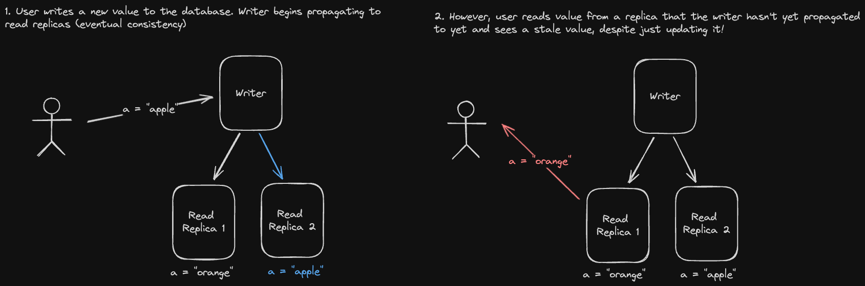
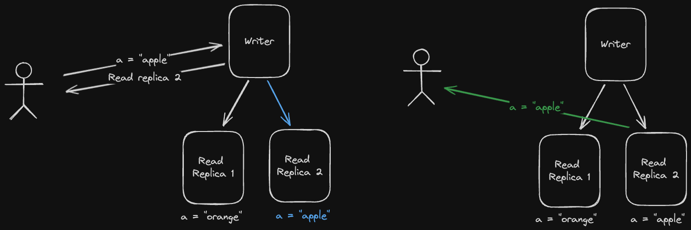
One way to mitigate this is to read your own writes:
- Whenever you write to a database replica, read from the same replica for some X time.
- Set X based on how long it takes to propagate that write to other replicas so that once X has passed, we can lift the restriction.
Another issue we could run into is if we read from replicas that are progressively less updated, resulting in reading data "out of order". Let's look at an example:
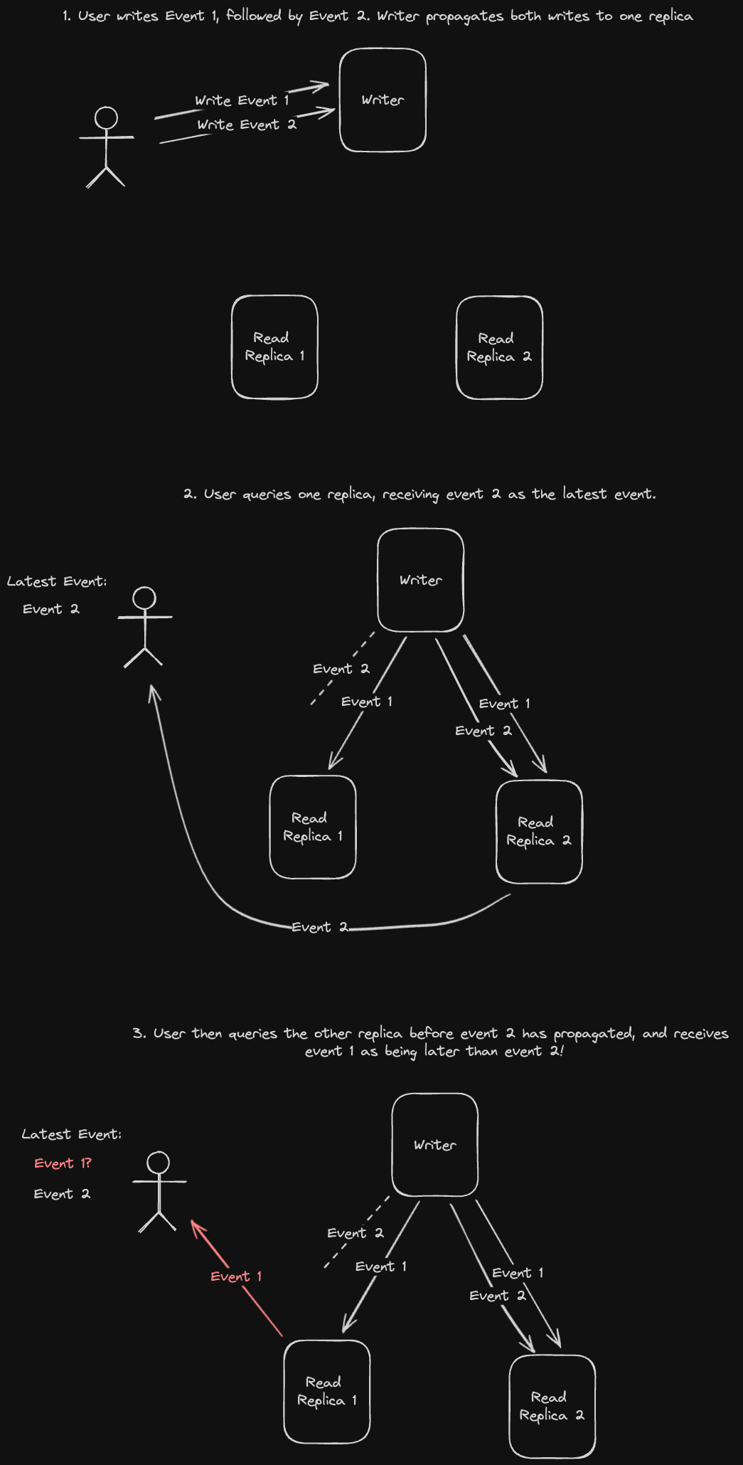
A possible solution for this is to have each user always read data from the same replica. This guarantees that our reads are monotonic reads - we might still read stale data from the same replica, but at least it will be in the correct order.
In a single leader replication (sometimes referred to as Master-Slave or Active-Passive), we designate a specific replica node in the database cluster as a leader and write to that node only, having it manage the responsibility of propagating writes to other nodes.
This guarantees that we won’t have any write conflicts since all writes are processed by only one node. However, this also means we have a single point of failure (the leader) and slower write throughput since all writes can only go through a single node.
In single leader replication, follower failures are pretty easy to recover from since the leader can just update the follower after it comes back online. Specifically, the leader can see what the follower’s last write was prior to failure in the replication log and backfill accordingly.
However, leader failures can result in many issues:
- The leader might actually be up, but the follower’s unable to connect due to network issues, which would result in it thinking it needs to promote itself to be the new leader
- A failure might result in lost writes if the leader was in the middle of propagating new writes to followers.
- When a leader comes back online after a new leader has already been determined, we could end up with two leaders propagating conflicting writes as clients send writes to both nodes (Split brain).
In general, single leader replication makes sense in situations where workloads are read-heavy rather than write-heavy. We can offload reads to multiple follower nodes and have the leader node focus on writes.
- Most relational databases like MySQL and PostgreSQL use single-leader replication. However, some NoSQL databases like MongoDB, AWS DynamoDB, and RethinkDB support it as well
- Some distributed message brokers like RabbitMQ and Kafka (which we'll talk about when we get to batch and stream processing), also support leader-based replication to provide high availability
In multi-leader replication, we write to multiple leader nodes instead of just one. This provides some redundancy compared to single-leader replication, as well as higher write throughput. It especially makes sense, performance wise, in situations where data needs to be available in multiple regions (each region should have its own leader).
There are a few topologies for organizing our write propagation flow between leaders.
As the name suggests, leader nodes are arranged in a circular fashion, with each leader node passing writes to the next leader node in the circle
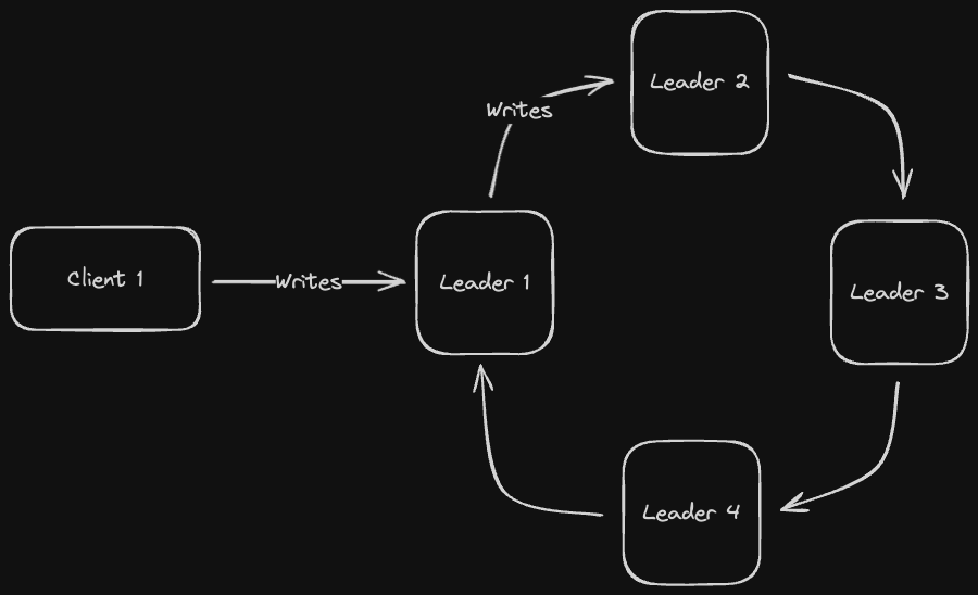
If a single node in the circle fails, the previous node in the circle that was passing writes no longer knows what to do. Hence, fault tolerance is non-existent in this topology
In a star topology, we designate a central leader node, which outer nodes pass their writes to. The central node then propagates these writes to the other nodes
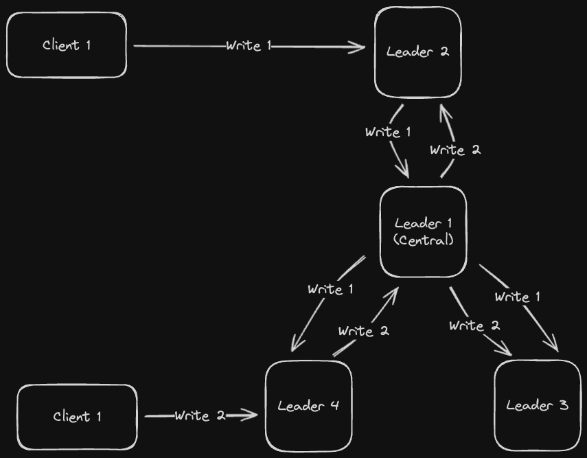
If the outer nodes die, we're fine since the central node can continue to communicate with the other remaining outer nodes, so it's a little bit more fault tolerant than the Circle Topology. But if the central leader node dies, then we're screwed
An all-to-all topology is a "complete graph" structure where every node propagates writes to every other node in the system (every node is the "central" node from the Star Topology)
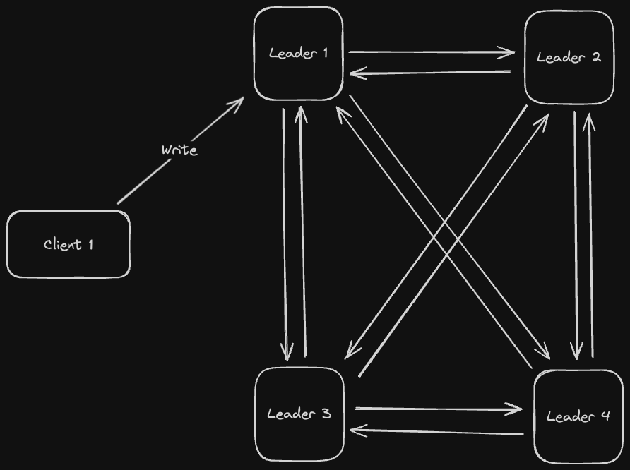
This is even more fault tolerant than the star topology since now if any node dies, the rest of the nodes can still communicate with each other. However, there are still some issues with this toplogy:
- Since writes are being propagated from every node to every other node, there could be cases where duplicate writes get propagated out
- Writes might not necessarily be in order, which presents an issue if we have causally dependent writes (for example, write B modifies a row created by write A)
There are some ways to mitigate these issues. We can fix the duplicates issue by keeping track in our Replication Log which nodes have seen a given write
Multi leader replication could result in concurrent writes that are unaware of each other, causing inconsistency in the database (write conflicts). There are a few solutions for mitigating this
As the name implies, conflict avoidance just has us avoid conflicts altogether by having writes for a particular key only go to one replica. This limits our write throughput, so it's not ideal
In a last-write wins conflict resolution strategy, we use the timestamp of the write to determine what the value of a key should be. The write with the latest timestamp wins
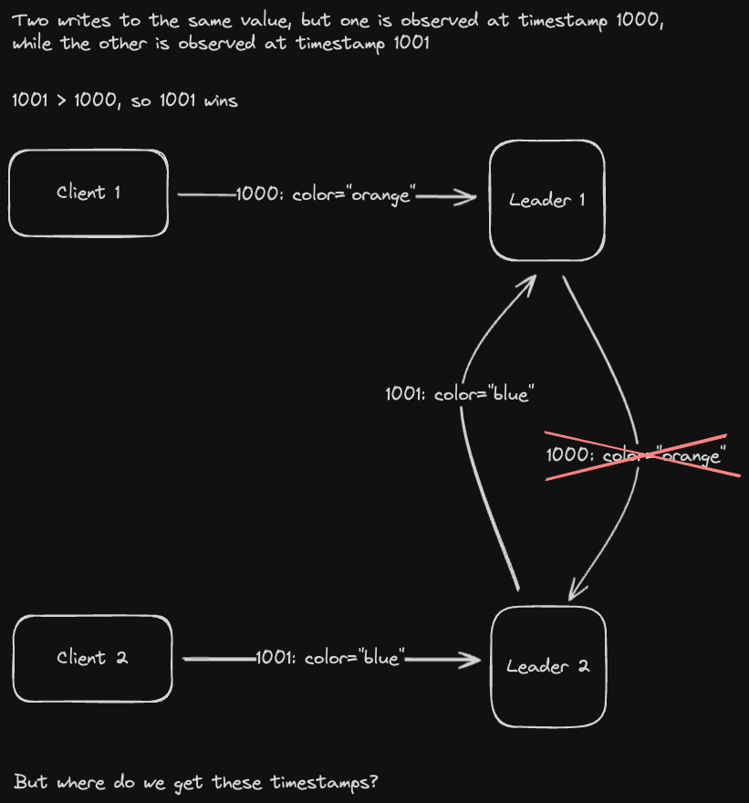
Determining what timestamp to use can be tricky - for one thing, which timestamp do we trust? Sender timestamps are unreliable since clients can spoof their timestamp to be years in the future and ensure their write always wins.
Receiver timestamps, surprisingly, can also be unreliable. Computers rely on quartz crystals which vibrate at a specific frequency to determine the time. Due to factors like weather conditions and natural degredation, these frequencies can change. This results in computers having slightly different clocks over time, a process known as clock skew
- There are some ways to mitigate clock skew, such as using Network Time Protocol (NTP) to get a more accurate timestamp from a time server using a GPS clock.
- However this solution isn't perfect since we're subject to network delays if we're making requests to servers
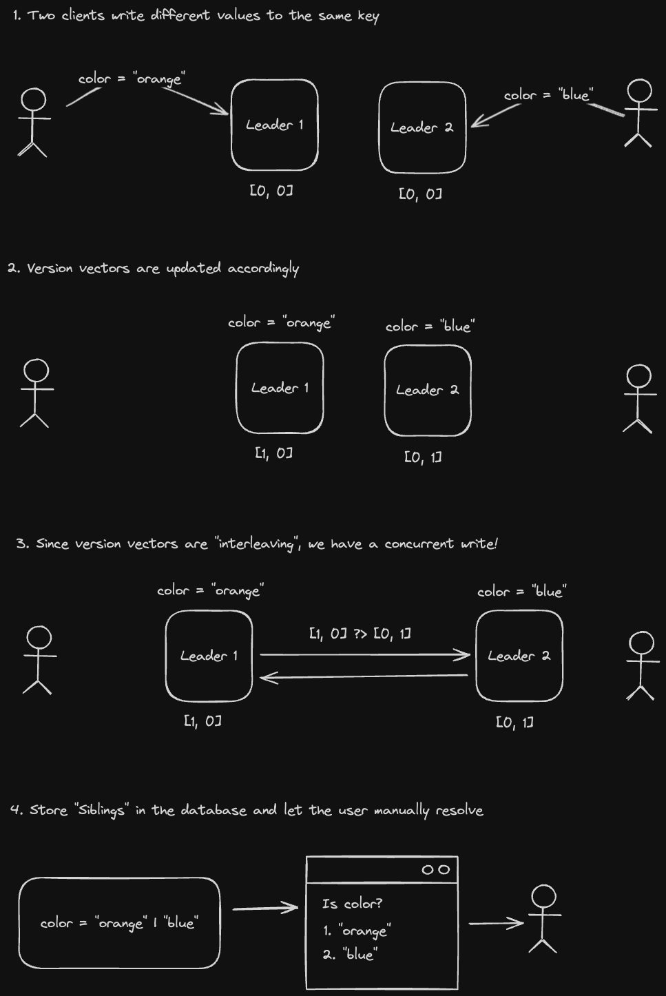
A version vector is just an array that contains the number of writes a given node has seen from every other node. For example, [1, 3, 2] represents "1 write from partition 1, 3 writes from partition 2, and 2 writes from partition 3"
We then use this vector to either merge data together and resolve the conflict or store sibling data and offload conflict resolution to the client. Let's look at an example:
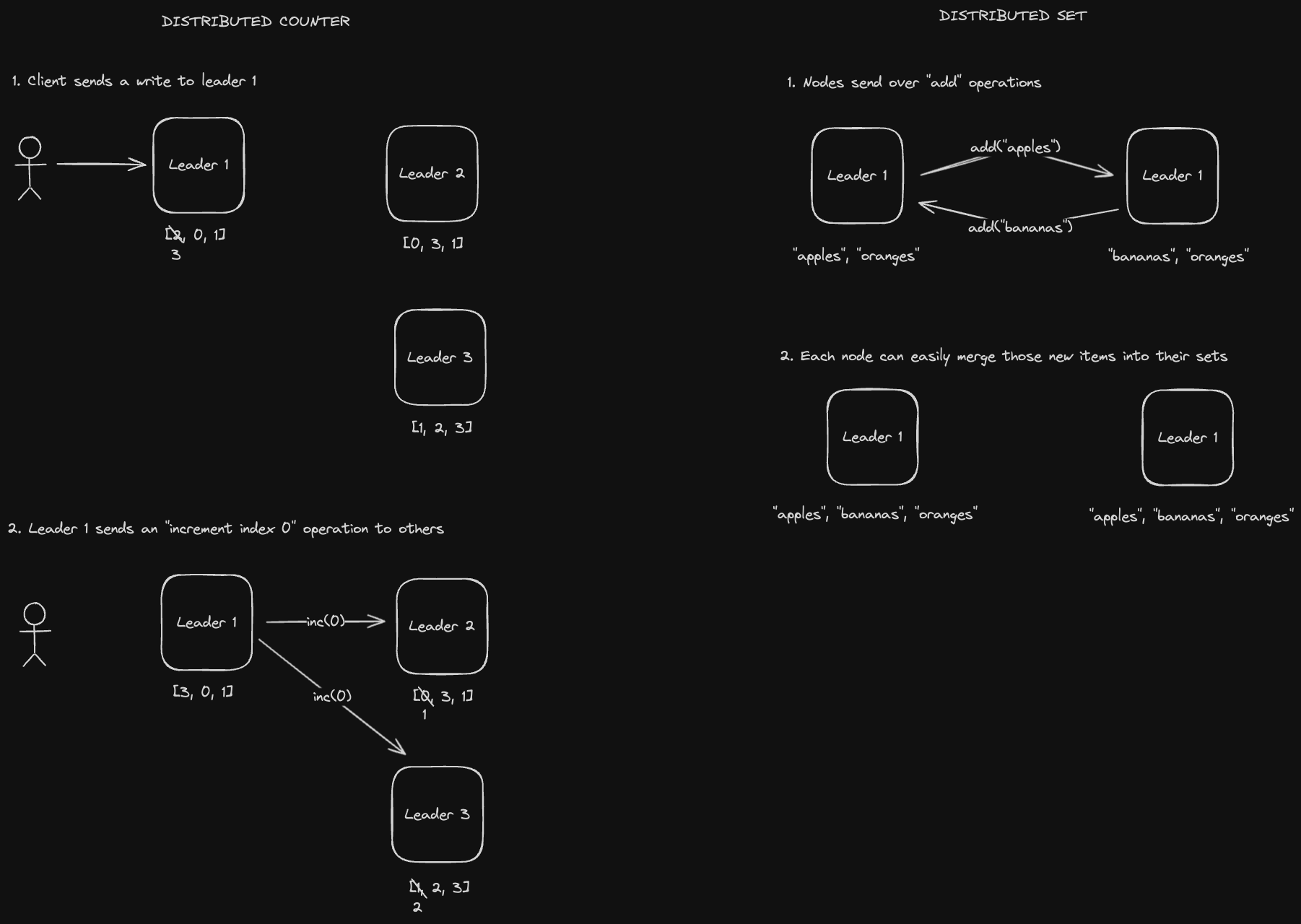
CRDTs are special data structures that allow the database to easily merge data types to resolve write conflicts. Some examples are a counter or a set.
Database nodes send operations to each other to keep their data in sync. These have some latency benefits compared to state-based CRDTs since we don't need to send as much data over the network.
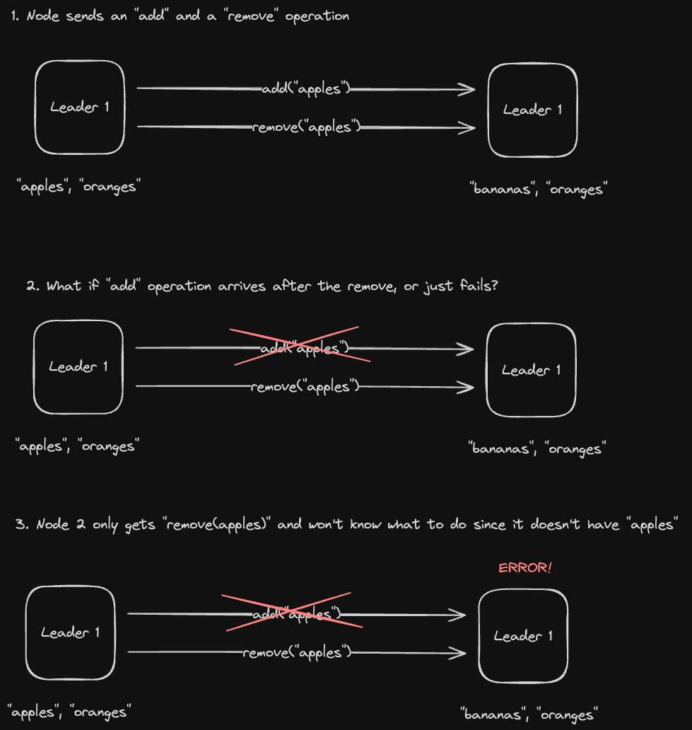
However, there are a few problems with Operational CRDTs. For one thing, they're not idempotent, so don’t do well when we have duplicate or dropped requests. For example in the distributed counter above, if we sent that increment operation multiple times due to some kind of failure / retry mechanism, we could have some issues.
Furthermore, what if we have causally dependent operations? For example:
Database nodes send the entire CRDT itself, and the nodes "merge" states together to update their states. The "merge" logic must be:
- Associative:
f(a, f(b, c)) = f(f(a, b), c) - Commutative:
f(a, b) = f(b, a) - Idempotent:
f(a, b) = f(f(a, b), b)
Let's take a look at an example.
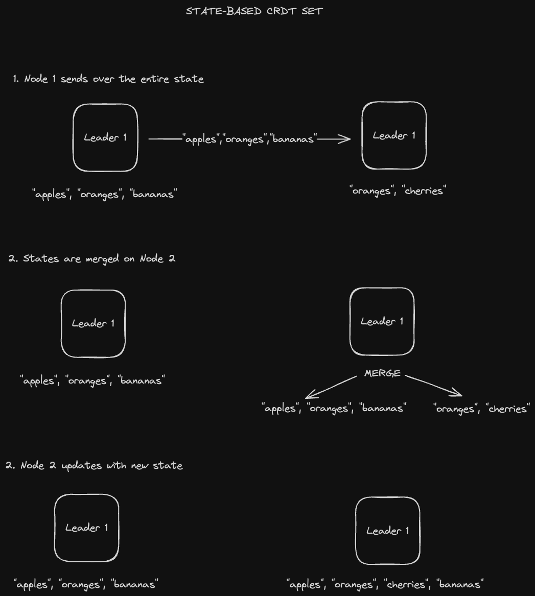
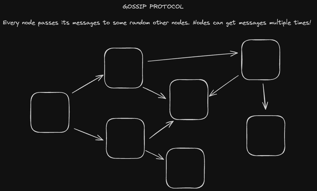
We can see that Node 1 sending that set multiple times would result in the same merged result on Node 2. This idempotency also enables state CRDTs to be propagated via the Gossip Protocol, in which nodes in the cluster send their CRDTs to some other random nodes (which may have already seen the message).
- CRDTs are used by systems like Redis (an in-memory cache) and Riak (a multi-leader/leaderless distributed key-value store).
Leaderless replication forgoes designating specific nodes as leader nodes entirely. In leaderless replication, we can write to any node and read from any node. This means we have high availability and fault tolerance, since every node is effectively a leader node. It also gives us high read AND write throughput.
To guarantee that we have the most recent values whenever we read from the system, we need a quorum, which just means "majority"
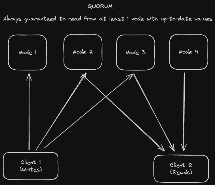
Writers write to a majority of nodes so that readers can guarantee that at least one of their return values will be the most recent when they read from a majority of nodes. In mathematical terms:
W (## of nodes we write to) + R (## of nodes we read from) > N (## of total nodes)
A nifty trick we can also do with quorums is read repair. Whenever we read values from R nodes, we might see that some of the results are out of date. We can then write the updated value back to their respective nodes.
There are some issues with quorums:
- We can still have cases in which writes arrive in different orders to a majority of nodes, causing disagreement amongst them as to which one is actually the most recent.
- Writes could also just fail, violating that inequality condition we just defined.
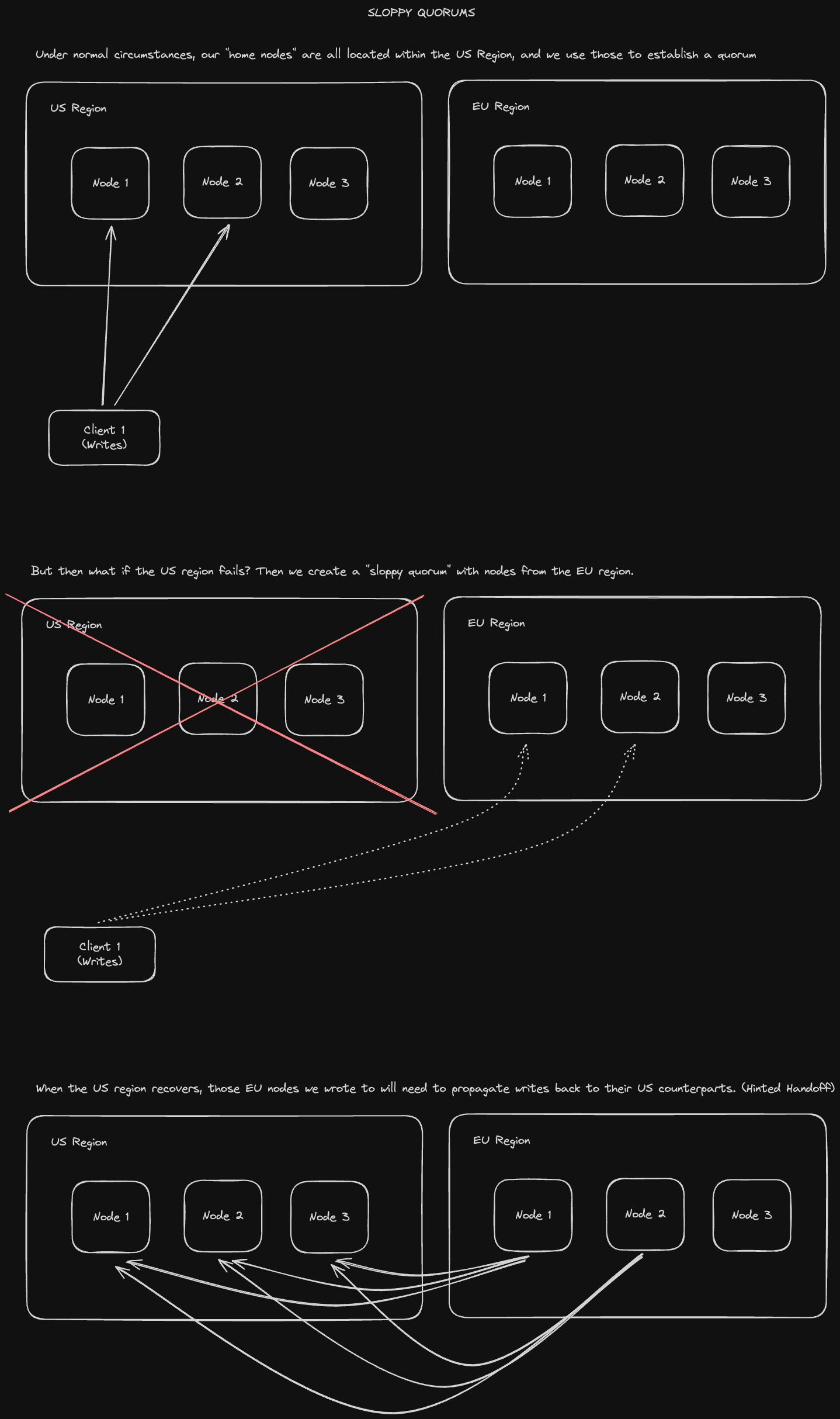
Let's imagine a client is able to talk to some database nodes during a network interruption, but not all the nodes it needs to assemble a quorum. We have two options here:
- Return errors for all requests for which we can't reach a quorum of nodes
- Accept writes anyways, but write them to nodes that are reachable, but which aren't necessarily the nodes that we normally write to.
The 2nd option causes a sloppy quorum where the W and R in our inequality aren't among the designated N "home" nodes. Once the original home nodes come back up, we need to propagate the writes that were sent to those temporary writer nodes back to those home nodes. This process is called hinted handoff. Let's take a look at an example:
Another way to prevent stale reads is to propagate writes in the background between nodes. For example, if node A has writes 1, 2, 3, 4, 5, and node B only has writes 2, 3, 5, we'd need the first node to send writes 1 and 4 over.
One way to do this is to just send the entire replication log with all the writes from node A. But this would be inefficient since all we need is the diff (just writes 1 and 4).
We can quickly obtain this diff using a Merkle Tree, which is a tree of hashes computed over data rows. Each individual row gets hashed to a value, and those values are combined and hashed hierarchically until we get a root hash over all the rows.
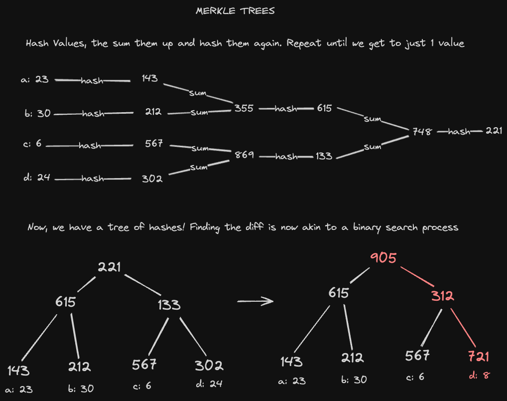
Using a binary tree search, we can efficiently identify what's changed in a dataset by comparing hash values. For example, the root hash will tell us if there is any change across our entire data set, and we can examine child hashes recursively to track down which specific rows have changed.
- Amazon's Dynamo paper popularized the leaderless replication architecture. So systems that were inspired by it support leaderless replication:
- Apache Cassandra
- Riak
- Voldemort, a distributed key-value store designed by LinkedIn for high scalability
- Interestingly, AWS DynamoDB does NOT use leaderless replication despite having Dynamo in the name
- Designing Data-Intensive Applications, Chapter 5, "Replication"
- jordanhasnolife System Design 2.0 Playlist:
- EnjoyAlgorithms System Design Blog:
Once our database starts getting too large, we'll need to split the data up across different pieces (partitions). Complications will arise in terms of how we should best split the partition, identifying partitions that a query should be routed to, and re-partitioning in the event of failure.
For choosing partitions, we have some different options:
- Range-based partitioning: Divide our data into ranges (of timestamp or name in alphabetical order, for example).
- Enables very fast range queries due to data locality.
- Could result in hot spots if a particular range is accessed more often than another.
- Hash-range based partitioning: Hash the key and assign it to a partition corresponding to the hash.
- Provides a more even distribution of keys, preventing hot spots.
- Range queries are no longer as efficient since we don’t have data locality (but we can mitigate this using indexes).
Federation (or functional partitioning), splits up databases by function. For example, an e-commerce application like Amazon could break up their data into users, reviews, and products rather than having one monolothic database that stores everything.
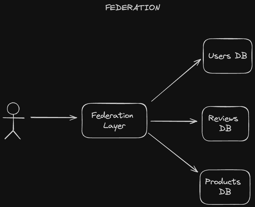
Federated databases are accompanied by a Federated Database Management System (FDBMS), which sits on top of the various domain-specific databases and provides a uniform interface for querying and storing data. That means users can store and retrieve data from multiple different data sources with just a single query. In addition, each of these individual databases is autonomous, managing data for its specific function or feature independently of others. Thus, an FDBMS is known as a meta database management system.
Splitting up data in this manner enables greater flexibility in terms of the types of data sources that we use. Different functional domains can use different data storage technologies or formats, and our federation layer serves as a layer of abstraction on top. That also means we have greater extensibility. When an underlying database in our federated system changes, our application can still continue to function normally as long as that database is able to integrate with the federated schema.
Of course, having this federation layer adds additional complexity to our system, since we'll need to reconcile all these different data stores. Performing joins over different databases with potentially different schemas may be complex, for example. Furthermore, having to do all this aggregation logic could impact performance.
A secondary index is an additional index that's stored alongside your primary index, which might keep data in a different sort order to improve the performance of certain other queries which might not benefit from the sort order of the primary index. There are two main types of secondary indexes.
Local secondary indexes are indexes local to a specific partition on a particular column.
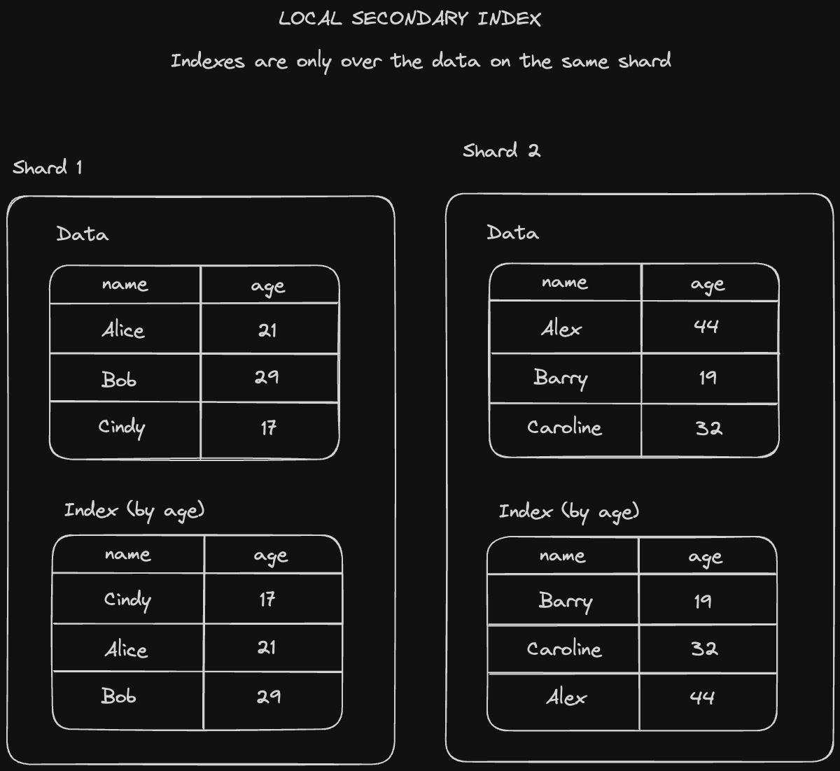
- Writing is fairly straightforward - every time we write a value to a partition, we also write it into the index on the same node.
- Reading is slower since we need to scan through the local secondary index of every partition and stitch together the result.
Global secondary indexes are indexes over the entire dataset, split up across our partitions.
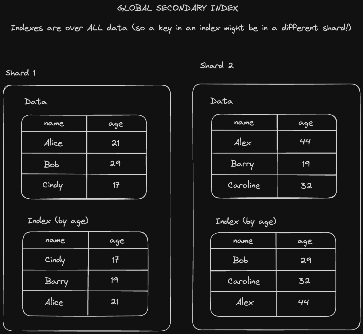
- Reading becomes much faster since we don’t need to query every single partition’s index. We can hone in on just the partitions that store whatever range we’re looking for.
- Writes will become slower since we might end up saving a key on two different partitions if the indexed location for that key is not in the same partition as its hash.
You might think a natural way to partition data is with the modulo operator. If we have 3 partitions, for example, every key gets assigned to the partition corresponding to the hash of that key modulo 3.
But then what if one of the partitions goes down? Then we need to repartition across our whole dataset since now every key should be assigned to the partition corresponding to its hash modulo 2.
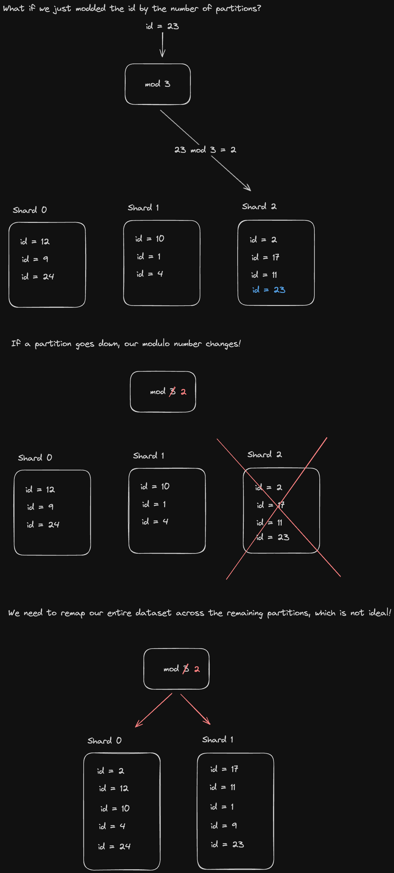
Is there some way we could rebalance the keys from only the partition that went down?
We can accomplish this through consistent hashing. In this scheme, we define hash ranges for every partition in such a way that whenever a partition goes down, we can extend the range for the remaining partitions to include the keys that were part of the partition that just went down.
In the event that the partition comes back online, we just reallocate those keys back to the partition in which they originally belonged.
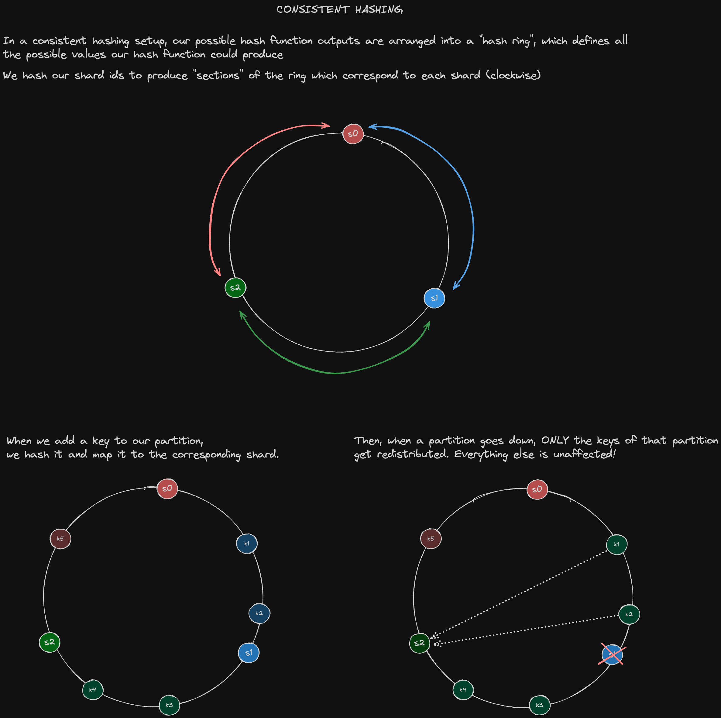
ByteByteGo also has a great video explanation of how this process works
We can also define a fixed number of partitions we have across our entire system rather than tying the number of partitions to the number of available nodes.
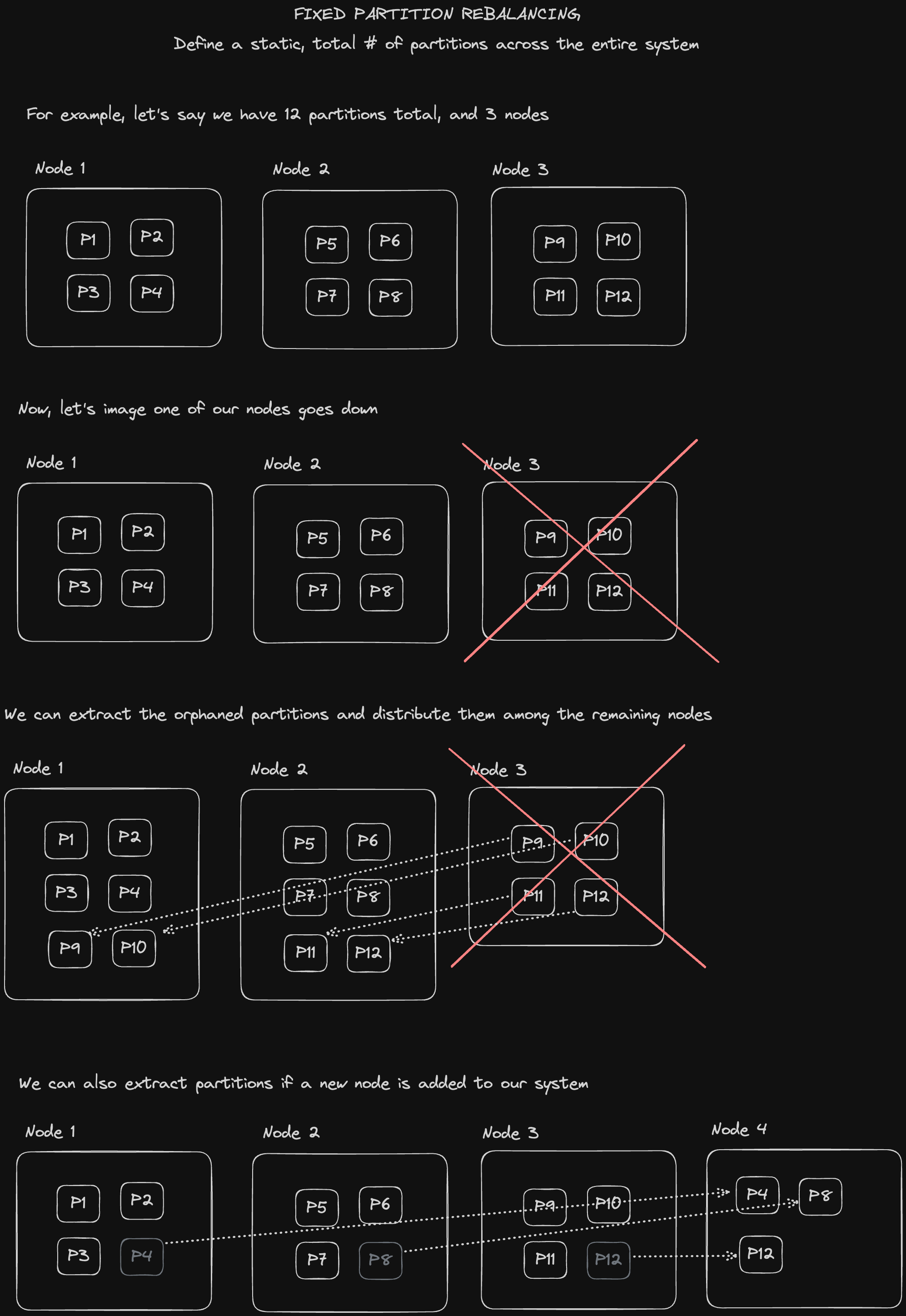
We can also utilize our system resources more effectively by distributing partitions to nodes according to their hardware capacity and performance, e.g. give more of the orphaned partitions to the more powerful machines.
A downside that might occur with this approach is that as our database grows, the size of each partition will grow in turn, since the total number of partitions is static. So that means we'd need to pick a good fixed partition number from the outset: one that isn't too large so as to make recovery from node failures expensive and complex, but also one that isn't too small so as to incur too much overhead.
- Designing Data-Intensive Applications, Chapter 6, "Partitioning"
- jordanhasnolife System Design 2.0 Playlist:
- Karan Pratap Singh's Open-source System Design Course: "Database Federation"
- Saurav Prateek: Systems that Scale: "Rebalancing Partitions Strategies"
As we saw with the eventual consistency of asynchronous replication schemes, there are no guarantees as to when consistency will actually be achieved. There are ways to mitigate this, but sometimes we value strong consistency guarantees over performance and fault tolerance.
Furthermore, an important abstraction that many distributed systems rely on is the ability to agree on something, or to come to a consensus. The key is to be able to do this effectively in the face of unreliable networks and failures.
Two Phase Commit is a way of performing distributed writes or writes across multiple partitions while guaranteeing the atomicity of transactions (writes either succeed on every partition or fail on every partition).
Writing to different partitions is unlike propagating writes across replicas because a single transaction to multiple partitions is effectively one logical write split up across multiple nodes. Hence this write needs to be atomic.
Two-phase commit designates a coordinator node to orchestrate the process. This node is usually just the application server performing the cross-partition write.
The following diagram describes the "happy case" flow for two-phase commit.
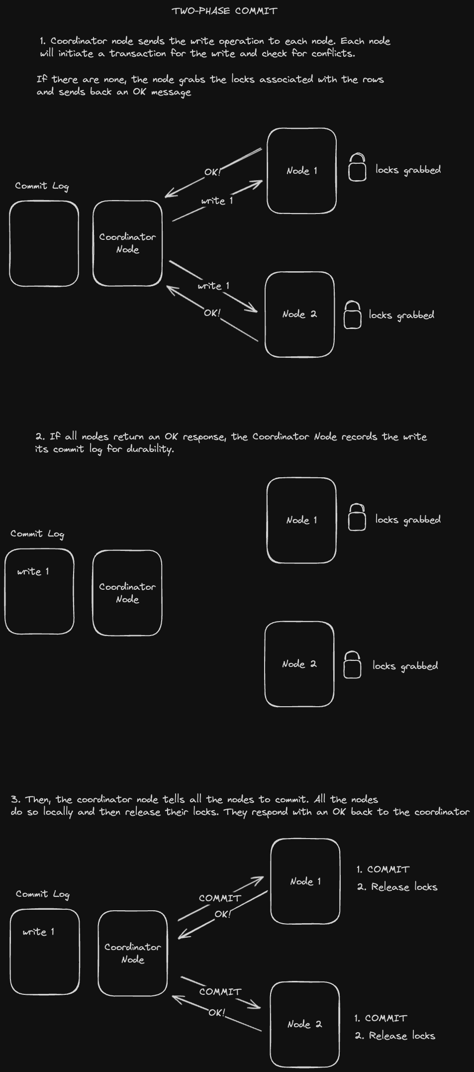
A few issues can arise:
- If a node is unable to commit due to a conflict, the coordinator node will need to send an ABORT command to that node and stop the entire process.
- If the coordinator node goes down, all the partition nodes will hold onto their locks, preventing other writes until the coordinator comes back online.
- If a receiver node goes down after the commit point, the coordinator node will have to send a request to commit repeatedly until the receiver comes back online.
We generally want to avoid 2PC whenever possible because it's slow and hard. So try to avoid writing across multiple partitions if possible.
Linearizable storage dictates that whenever we perform a read, we can never go back in time (we always read the most recent thing). In other words, we want to preserve the ordering of writes. This is important for determining who is the most recent person to obtain a lock in a distributed locking system or who is the current leader in a single leader database replication setup.
Coordination services like Zookeeper will need this to keep track of database replication leaders and the latest status of application servers, for example.
Let's take a look at how linearizable storage applies to different replication setups:
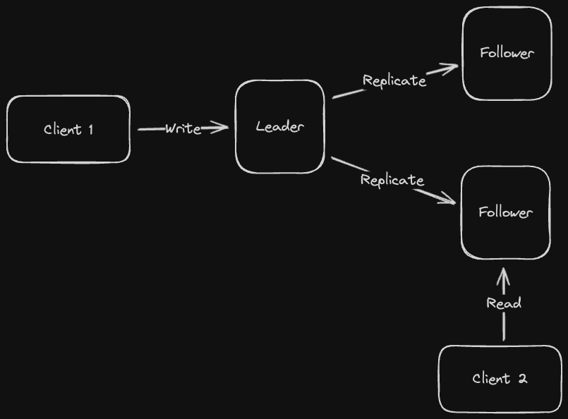
In single leader replication, log writes are guaranteed to be in order since we only have one writer node keeping track of everything. That seems like that would produce linearizable storage, right?
Turns out, not necessarily! If the client reads from the leader before it can replicate a new write over to a follower, and then goes down, that will force the client to read from the follower with an outdated value. So this isn’t actually linearizable storage.
In multi-leader or leaderless replication, writes can go to many places and we could have concurrent writes, so we can’t make any guarantees about maintaining a chronological ordering (or it doesn’t even make sense to). We should try to achieve a consistent ordering across all nodes instead
There are a couple of ways we might do this:
Version vectors
If we see a higher number of writes across all partitions for a given node, we can determine that version vector to be more recent. For example [1, 2, 1] is more recent than [0, 1, 0]
We can use some arbitrary mechanism for tie-breakers (interleaved version vector numbers). For example, we just pick the one with the higher left-most partition writes as being more recent.
Version vectors take O(N) space where N is the number of replicas, so it might not be the most efficient solution if we have a lot of replicas.
Lamport clocks
A Lamport clock is a counter stored across every replica node which gets incremented on every write, both on the client AND the database.
Whenever we read the counter value on the client side, we write back the max of the database counter and the client counter alongside the write. This value overrides the one on both the client and server, guaranteeing that all writes following this one will have a higher counter value. When sorting writes, we sort by the counter. If they’re the same, we can sort by node number. Let's see an example of how this might work:
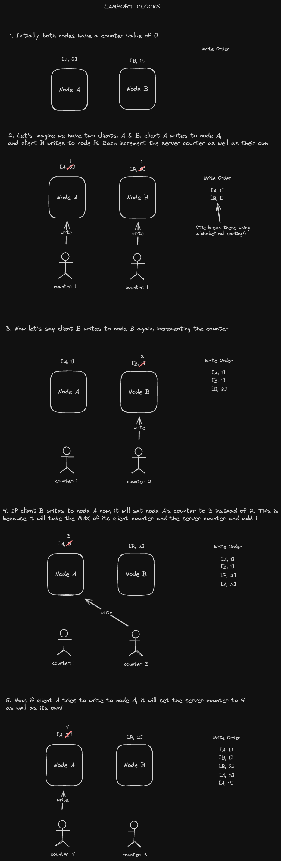
Unfortunately, we could still end up READING old data if replication hasn’t propagated through the system, so this isn’t actually linearizable storage. We only get ordering of writes after the fact.
CAP Theorem states that it's impossible for a distributed system to provide all three of the following:
- Consistency: The same response is given to all identical requests. This is synonymous with linearizability, in which we provide a consistent ordering of writes such that all clients read data in the same order regardless of which replica they're reading from. (Cruciallly it's NOT the same thing as Consistency in ACID)
- Availability: The system is still accessible during partial failures
- Partition Tolerance: Operations remain intact when nodes are unavailable.
Historically, CAP Theorem has been used to analyze database technologies and the tradeoffs associated with them. For example:
- "MongoDB's a CP database! its single leader replication setup enables it to provide consistent write ordering, but could experience downtime due to leader failures.".
- "Cassandra is an AP database! It has a leaderless or multi-leader replication setup that provides greater fault tolerance, but is eventually consistent in the face of write conflicts."
However, some have criticized CAP Theorem of being too simple (most notably, Martin Kleppmann, author of Designing Data-Intensive Applications).
Thus, the PACELC theorem attempts to address some of its shortcomings, preferring to frame database systems as either leaning towards latency sensitivity or strong consistency. it states:
"In the case of a network partition (P), one has to choose between either Availability (A) and Consistency (C), but else (E), even when the system is running normally in the absence of partitions, one has to choose between latency (L) and loss of consistency (C)"
The Raft distributed consensus protocol provides a way to build a distributed log that’s linearizable.
Below is the process for electing a new leader in Raft:
One node is designated as a leader and sends heartbeats to all of its followers. If a heartbeat is not received after some randomized number of seconds (to prevent simultaneous complaints), a follower node will initiate an election.
Follower node proposes itself as a candidate for the election corresponding to the next term.
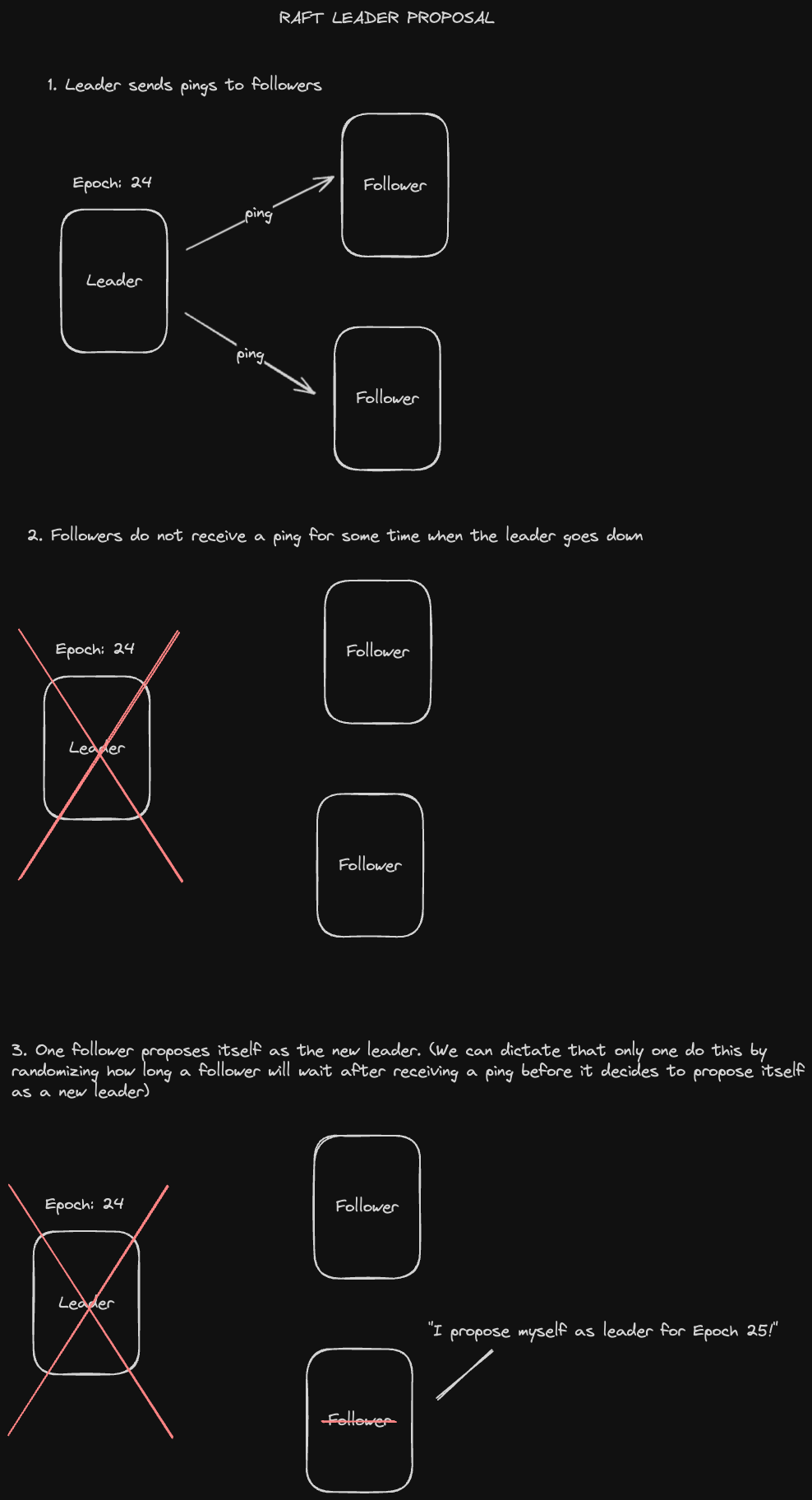
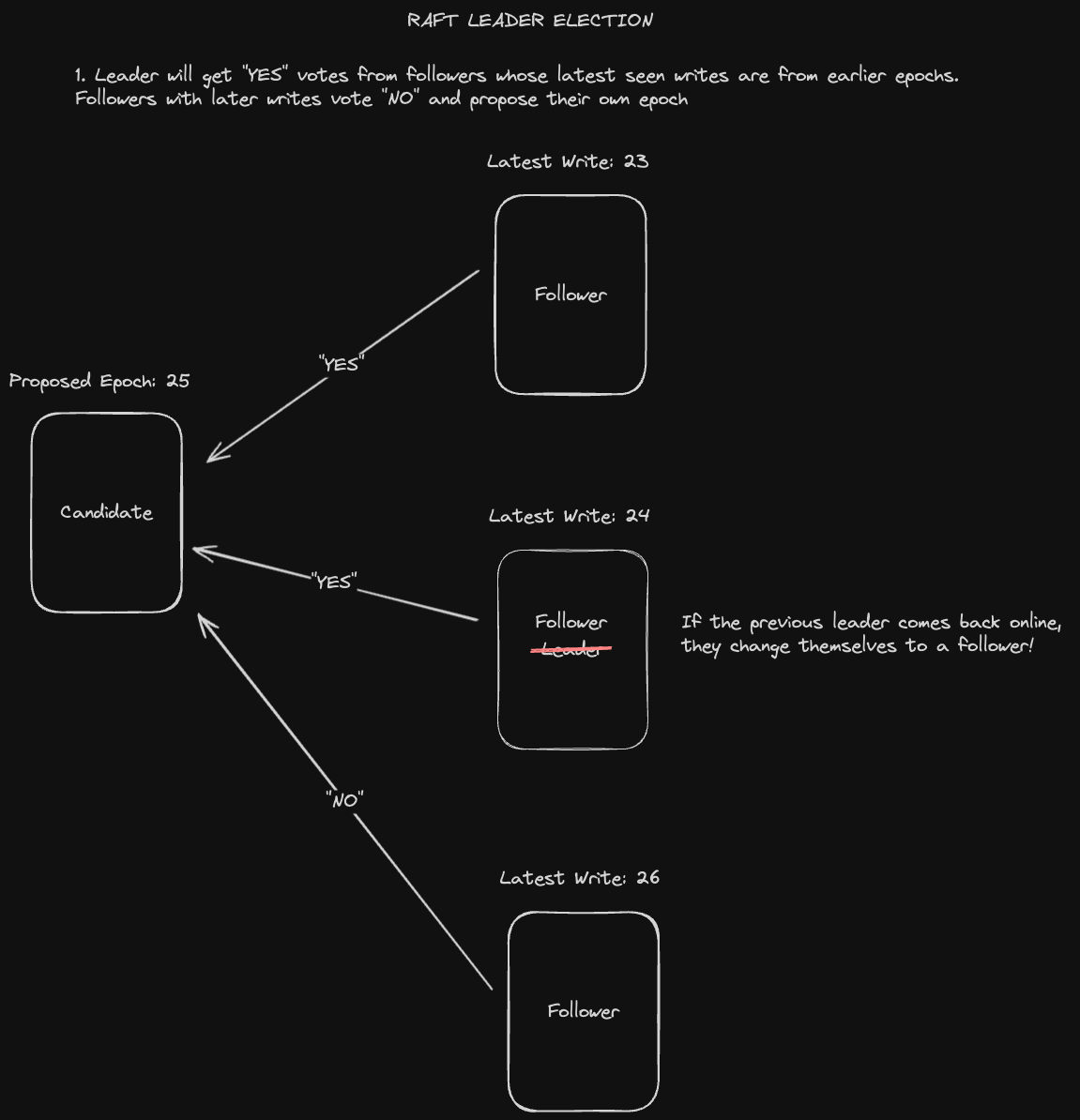
The election is held as follows:
- A follower from a previous term number (which is determined by the latest write that it’s seen) will change itself to a follower of the proposed term number and vote “yes”.
- A follower who has a write from a newer term number will vote “no” and also update its own term number value to the one being proposed if it is higher.
- If a candidate gets “yes” votes from a quorum of nodes, it wins the election and becomes the new leader.
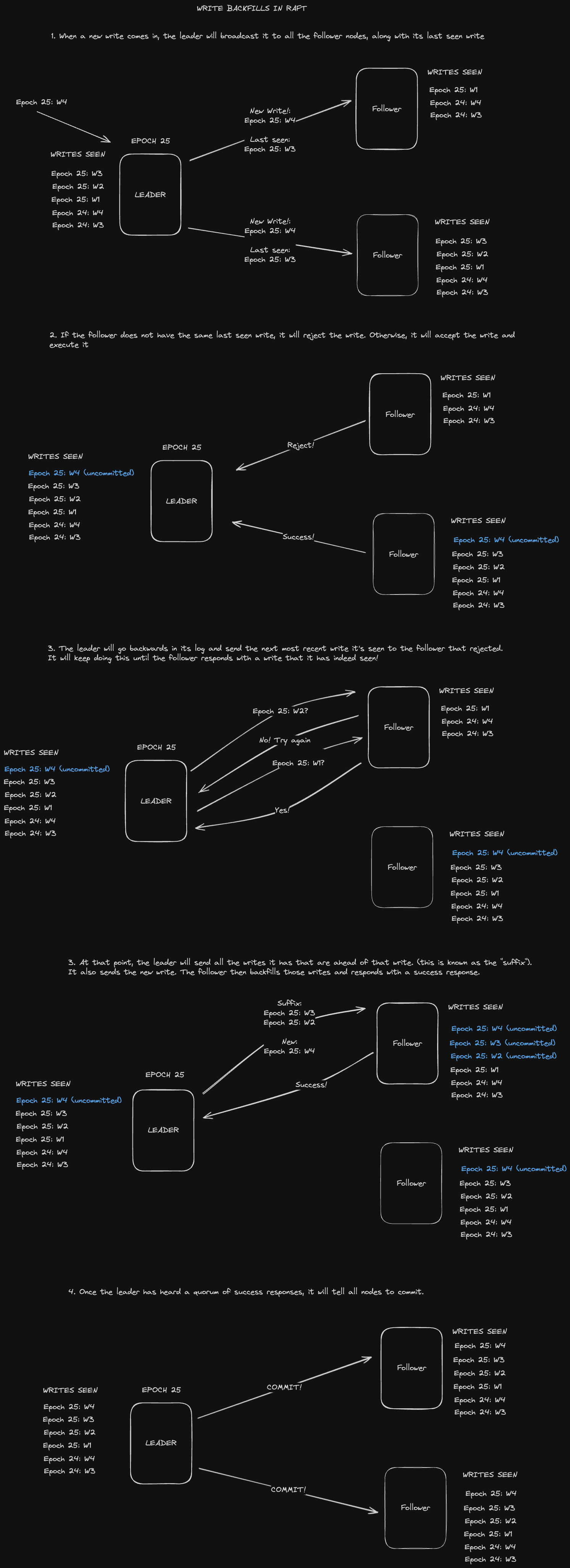
In Raft, we designate a leader that handles all writes. These writes are recorded in the form of logs, which contain an operation and a term number. Given the fact that only one node handles writes, it's possible that followers could have out of date logs.
Raft has 2 invariants when it comes to writes to address out of date logs:
- There is only one leader per term
- Successful writes must make the log fully up to date.
So writes backfill logs in addition to writing new values in order to keep them up to date. Furthermore, this invariant guarantees that if two logs are the same at a given point in time, every entry prior to that point will be the same
How does this actually work in practice? Let's look at a diagram of the process:
In conclusion, Raft is fault-tolerant and creates linearizable storage; however, it is slow and shouldn’t be used except in very specific situations where you need write correctness.
- Designing Data-Intensive Applications, Chapter 9, "Consistency and Consensus"
- jordanhasnolife System Design 2.0 Playlist:
- Martin Kleppmann, "Please stop calling databases CP or AP"
- Scylla DB Technical Glossary: "PACELC Theorem"
A cache is a hardware or software component that stores data so that future requests for that data can be served faster. In the context of an operating system, for example, we have CPU hardware caches set up hierarchically (L1, L2, L3) to speed up data access from main memory.
In distributed systems, caching provides several important benefits:
- Reduce load on key components
- Speed up reads and writes- caches typically store data on memory and are sometimes located physically closer to the client.
There are some challenges with caching - cache misses are expensive since we have to do a network request to the cache, search for the key and discover it’s missing, and then do a network request to the database. Furthermore, data consistency on caches is complex. If two clients each hit two different caches in two different regions, ensuring the data between the two is consistent can be a tough problem to solve.
We generally want to cache the results of computationally expensive operations. These could include database query results or computations performed on data by application servers.
We can also cache popular static content such as HTML, images, or video files. (We'll talk more about this when we get to CDNs)
-
Local on the application servers themselves
- This requires us to use consistent hashing in our load balancer to ensure requests go to the same server every time.
- Pros: Fewer network calls, very fast.
- Cons: Cache size is proportional to the number of servers.
-
Global caching layer
- Pros: Nodes in the global caching layer can be scaled independently.
- Cons: Extra network call, more can go wrong.
There are two popular choices for implementing application caches in software systems:
Memcached
Memcached is an open source distributed in-memory store. It uses an LRU eviction policy as well as consistent hashing for partitioning data, meaning the requests to the same key will be sent to the same partition.
Memcached is fairly bare-bones and is more useful for a customized caching implementation involving multi-threading or leaderless/multi-leader replication.
Redis
Redis is a more feature-rich in memory store, with support for specialized data structures like hash maps, sorted sets, and geo-indexes. It uses a fixed number of partitions, re-partitioning using the gossip protocol. It also supports ACID transactions using its write ahead log and single threaded serial execution. Its replication strategy uses a single leader.
There are a few different methods for writing to a distributed cache.
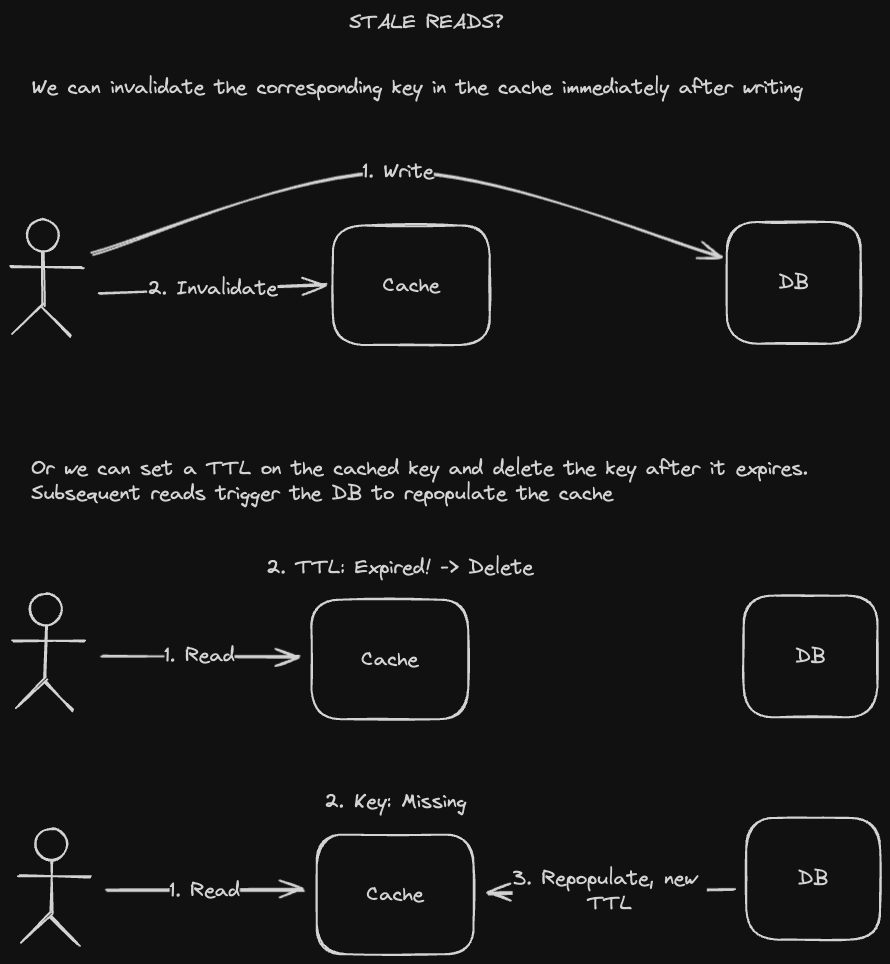
A write-around caching strategy entails sending writes directly to the database, going "around" the cache.
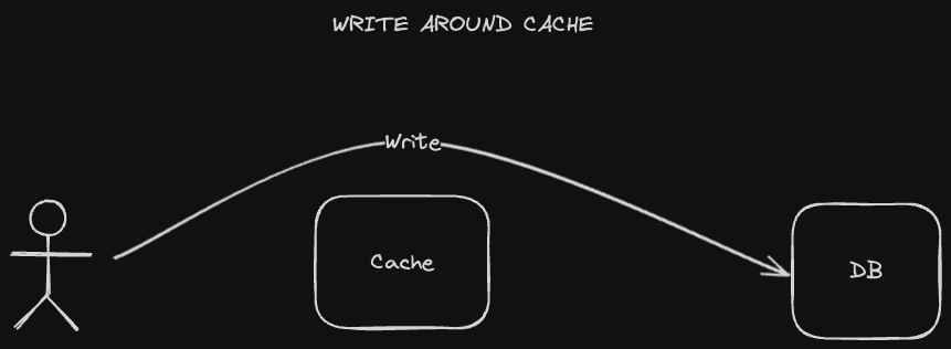
Of course, this means that the corresponding cached value will now be stale. We have a couple of ways to fix this:
-
Stale Read / TTL - We set a Time To Live (TTL) on the value in the cache, which is like an expiration date. Reads to the cache key will be stale until the TTL expires, at which point the value will be removed from the cache. A subsequent read on that key will go to the database, which will then repopulate the cache and set a new TTL
-
Invalidation - After writing to the database, we also invalidate its corresponding key in the cache. Subsequent reads will trigger the database to repopulate the cached value.
- Pros: Database is the source of truth, and writes are simple since they're not that different from our usual, non-cache flow
- Cons: Cache misses are expensive since we need to make 2 network calls, 1 for fetching the value from the cache and 1 for fetching the value from the database.
A write-through caching strategy is when we send writes to the cache, then proxy that request to the database. This means we may have inconsistent data between our cache and our database. Sometimes that isn't an issue, but in the cases where it is, we'd need to use two phase commit (2PC) to guarantee correctness.
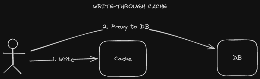
- Pros: Data is consistent between the cache and the database.
- Cons: Correctness issues if we don’t use 2PC. If we do, 2PC is slow.
A write-back caching strategy is similar to the write-through caching strategy, except writes aren’t propagated to the database immediately. We do this mainly to optimize for lower write latency since we’re writing to the cache without having to also write to the database. The database write-back updates are performed asynchronously - at some point down the line, or maybe on a fixed interval, we group writes in the cache and send them to the database together.
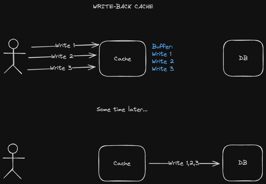
There are a few problems that could occur - for one thing, if the cache just fails, then writes never go to the database and we have incorrect data. We can provide better fault tolerance through replication, though this may add a lot of complexity to the system.
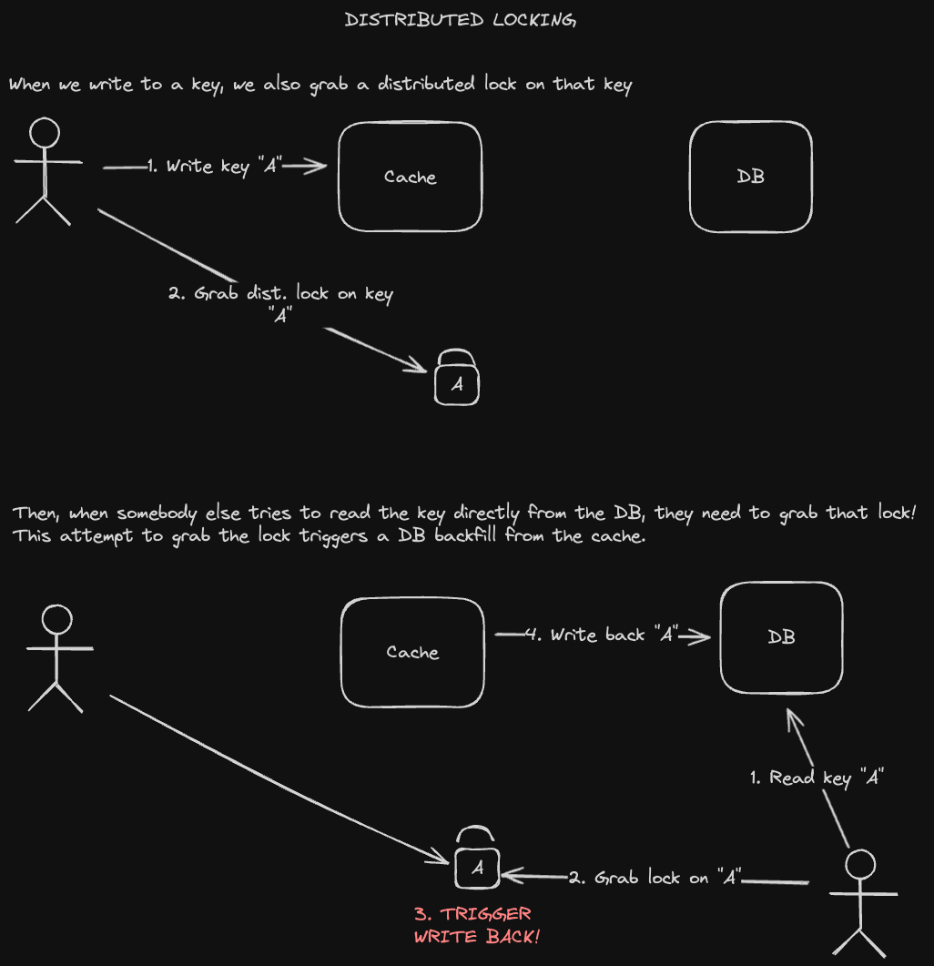
Furthermore, if a user tries to read directly from the database before the write backs can happen, they may see a stale value. We can mitigate this with a distributed lock:
- Whenever we write to the key in our cache, we also grab the distributed lock on that key.
- We hold the lock until somebody tries to also grab that lock while reading that key in the database.
- This other attempt to grab the lock would trigger a write back from the cache to the database, allowing the reader to see the up to date value.
Here's a diagram of that process:
Again, this adds a lot of complexity and latency, so we typically try to avoid needing to do this.
- Pros: Low latency writes.
- Cons: We may have stale or incorrect data
Our caches have limited storage space, so we'll need to figure out how best to manage what's stored in the cache and how to get rid of things. Our aim is to minimize cache misses, so let's take a look at how we can best do that.
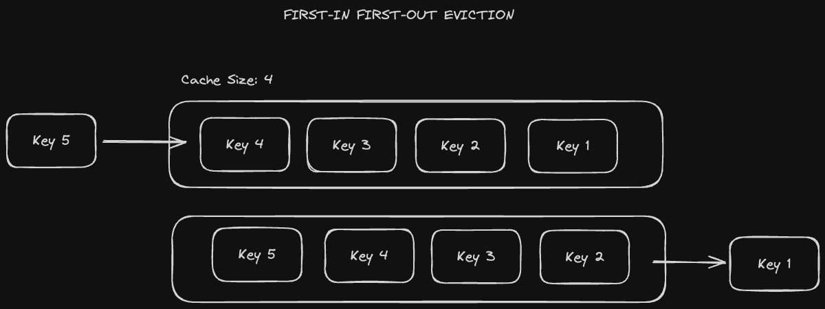
The first value in the cache becomes the first value to be evicted. It's relatively simple to implement since it's basically a queue. Every time we add a new value to the cache, we delete whatever the oldest value in the cache was.
The major problem with this is that we don't consider data access patterns and might evict data that's still actively being queried. For example, even if many users are querying a specific key, that key will eventually become the oldest key added to the cache as new data is added. It will subsequently be evicted despite being the most popular key.
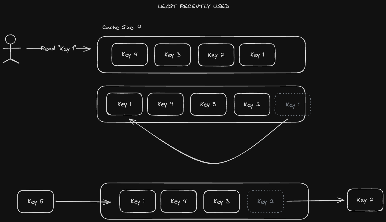
A better policy for evicting data is the "Least Recently Used" (LRU) policy. This is the most commonly used eviction policy in practice. In LRU, the last accessed key gets evicted, and more recently used keys get to stay in the cache. This solves the problem we saw earlier with First-in First-out - popular keys will remain cached since they will keep being used.
LRU is a bit more complicated to implement - rather than just having a queue we'd need to use a hashmap with a doubly linked list. We need a hashmap to identify the node to move to the head of the list, and a doubly-linked list to be able to shift things around in O(1) time.
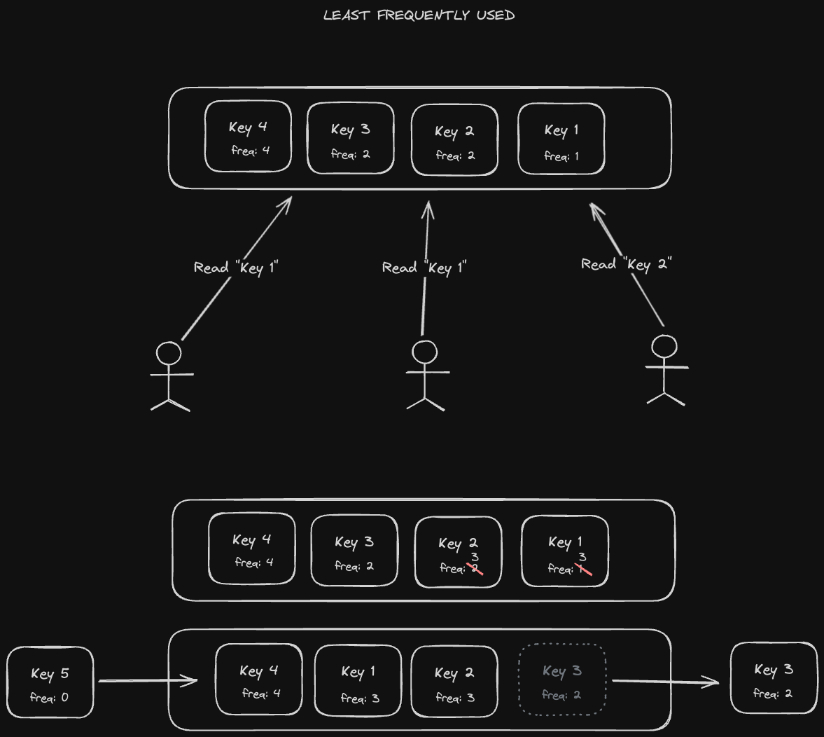
A more sophisticated alternative is "Least Frequently Used", where we keep track of the frequencies that a key is being accessed and evict according to that.
Using this policy alone also has some problems - if a key is referenced repeatedly for a short period of time and then not touched for a long time afterwards, it might stay in the cache simply because it has a high frequency count from that initial spike in popularity. In addition, new items in the cache might be removed too soon since they start with a low frequency counter.
Therefore, an LFU policy is typically best for situations in which access patterns of cached objects do not change often. For example, the Google logo will always be accessed at a fairly high rate, but a hype storm around a new logo for Instagram or Reddit might temporarily increase its recency in the cache. Once the hype dies down, those new logos will be evicted as their frequency count stops growing, while Google's remains in the cache.
Content Delivery Networks (CDNs), are geographically distributed caches for static content, like HTML, image, video, and audio files. These files tend to be large, so we'd like to avoid having to download them repeatedly from our application servers or object stores (which we'll get into later).
There are a couple of types of CDNs:
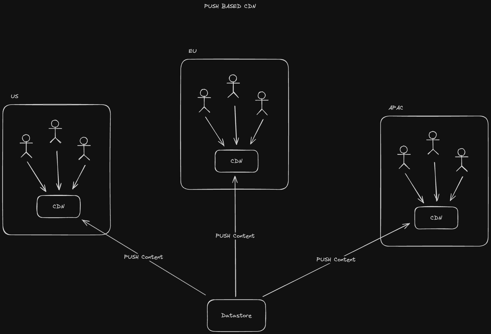
A push CDN pre-emptively populates content that we know will be accessed in the CDN. For example, a streaming service like Netflix may have content that comes out every month that they'd anticipate their subscribers will consume, so they pre-load it onto their CDNs
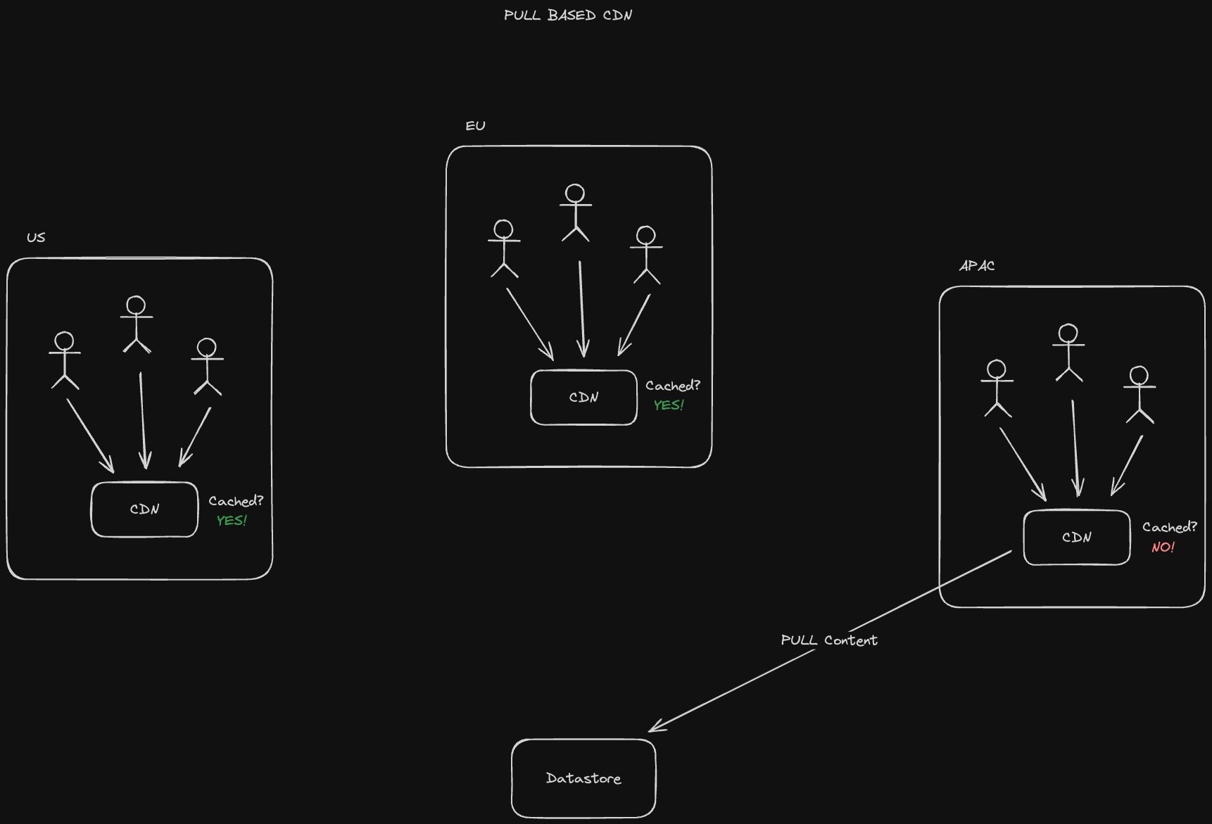
A pull CDN, in contrast, only populates the CDN with content when a user requests it. These are useful for when we don’t know in advance what content will be popular.
- Akamai provides CDN solutions among other edge computing services
- Cloudflare provides a free CDN service
- AWS CloudFront is AWS's CDN offering
- Ilija Eftimov's Blog "When and Why to use an LFU cache with an implementation in Golang"
- jordanhasnolife System Design 2.0 Playlist:
Batch processing is the method computers use to periodically complete high volume, repetitive data jobs. Certain data processing tasks like backups, filtering, and sorting are compute intensive and inefficient to run on individual data transactions. Let's take a look at some of the systems we generally use to accomplish this.
Hadoop is a distributed computing framework that is used for data storage (Hadoop Distributed File System) and batch processing (MapReduce or Spark).
The Hadoop Distributed File System, or HDFS, is a distributed, fault tolerant file store that's "rack aware". That means that we take into account the location of every computer we're storing data on in order to minimize network latency when reading and writing files.
The architecture of HDFS has two main elements: Name Nodes, which are used for keeping track of metadata, and Data Nodes, which are used for actually storing the files.
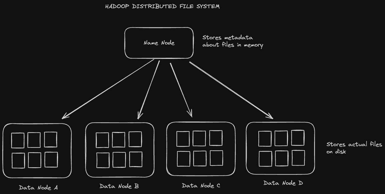
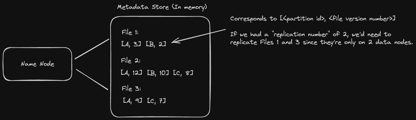
Every name node keeps track of metadata telling us which data node replicas store a given file, along with what version of the file the replicas have. This metadata is stored in memory (for read performance) with a write ahead log saved on disk for fault tolerance.
When a name node starts up, it asks every data node what files it contains and what versions they are. Based on this information, it replicates files to data nodes using a configurable "replication number". For example, if we setup HDFS to use a replication number of 3 and the name node sees that a file is only stored on 2 data node replicas, it will go ahead and replicate that file to a 3rd data node.
Generally we expect to read data from HDFS more often than we write it. The reading process is as follows:
- A client asks a name node for the file location
- The name node replies with the best data node replica for the client to read from
- The client caches the data node replica location
- The client reads the file from that data node replica
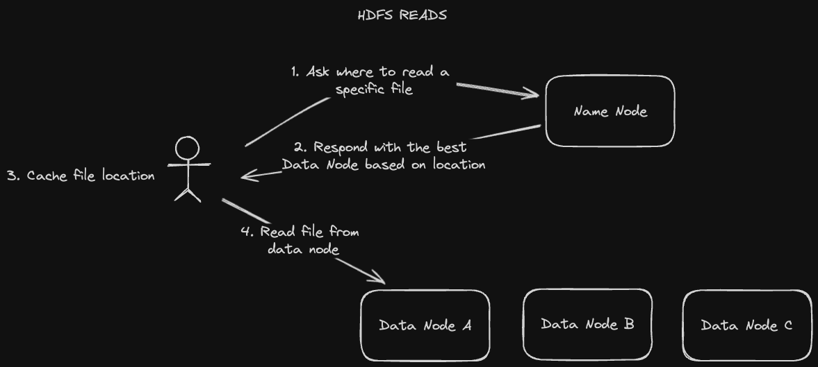
The "rack awareness" feature comes into play in step 2. The name node determines which replica is best for the client based on the client's proximity to it. Once the client receives that information, it can just save it in its cache rather than having to ask the name node every time.
When we write to HDFS, the name node has to select the replica it writes to in a "rack aware" manner. Here's how that plays out when we're writing a file for the first time:
- A client tells the name node it wants to write a file
- The name node will respond with a primary, secondary, and tertiary data node to the client based on ascending order of proximity
- The client will write their file to the primary data node
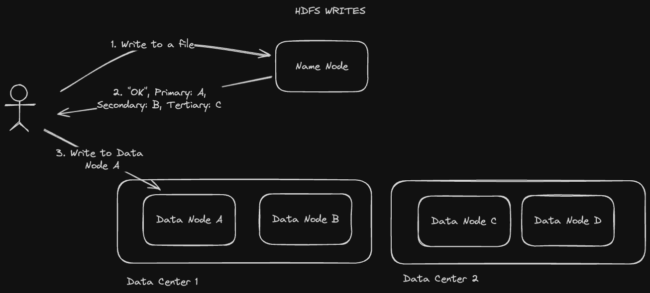
The name node will replicate across data nodes that might be in the same data center in order to minimize network latency. For example, the primary and secondary data nodes it responds with in step 2 may be in one data center, with the tertiary data node in another.
Notice that the client only writes to one data node in the previous example. HDFS propagates the file to the secondary and tertiary data nodes in a process known as "replication pipelining". This process is fairly straightforward: every replica will write to the next replica in the chain, e.g. primary writes to secondary, secondary writes to tertiary. On each successful write, an acknowledgement will be received. Under normal circumstances, the acknowledgement will propagate its way back to the client when the replication has succeeded across all data nodes.
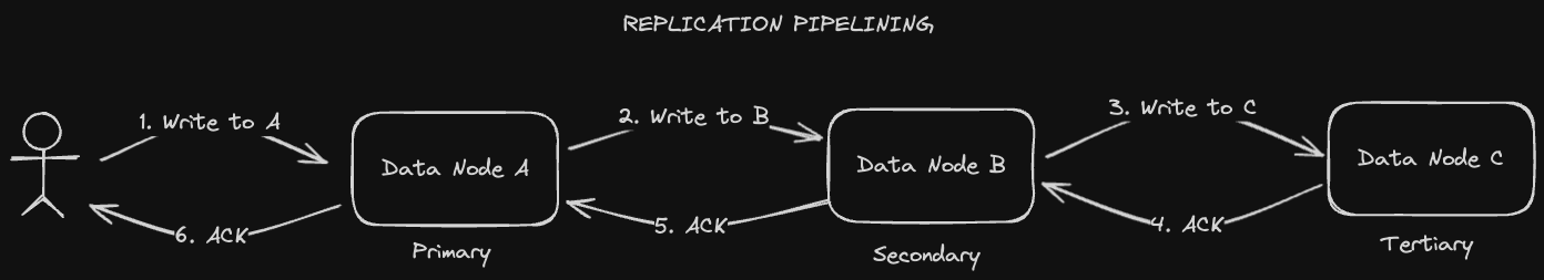
If there's a network failure between a primary and a secondary data node for example, the client won't receive this acknowledgement and data might not successfully replicate. The client at this point can accept eventual consisteny, or it can continue to retry until it receives that acknowledgement. However, it's not guaranteed that that acknowledgement will ever be received. As a result, HDFS cannot be called strongly consistent.
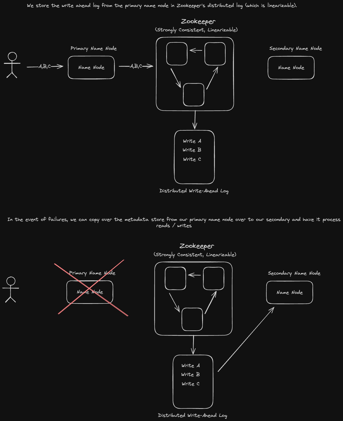
Name nodes represent a single point of failure in our system if we only have one of them. HDFS solves for this issue by using a coordination service like Zookeeper to keep track of backup name nodes. Coordination services are strongly consistent via the use of distributed consensus algorithms.
If a primary name node fails, its write ahead log operations stored in Zookeeper, will be replayed to the secondary name node to reconstruct the metadata information in memory. That secondary name node will then be designated as the new primary name node. This replay process is known as state machine replication.
The Problem with HDFS
One problem with HDFS is that modifying a single value in a file is very inefficient. In order to change one key, for example, we'd need to overwrite the entire file, which could be on the order of megabytes in terms of size. This is extremely expensive, especially when you factor in replication.
Apache HBase, an open-source database built on top of HDFS, can help us solve this problem. It allows for quick writes and key updates via LSM trees, as well as good batch processing functionality due to data locality from column oriented storage and range based partitioning, which keeps data with similar keys on the same partition.
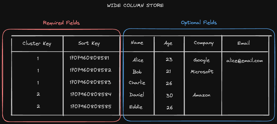
Data Model
HBase, similar to Apache Cassandra, is a NoSQL Wide Key Store. Recall that a wide-column database organizes data storage into flexible columns that can be spread across multiple servers or database nodes. Each row has a required cluster and sort key, and every other column value after that is optional.
Architecture
Similar to HDFS, HBase maintains master nodes and partition nodes. The master node provides the same functionality as a name node in HDFS, storing metadata about data nodes and directing clients who want to read and write to their optimal data node.
The partition node, however, contains an HDFS data node as well as a region node. The region node stores and operates the LSM Tree in memory and flushes it to an SSTable stored in the data node when it gets to a certain capacity. The data node, as we saw in the HDFS section, will then replicate these SSTables to other data nodes in the replication pipeline.
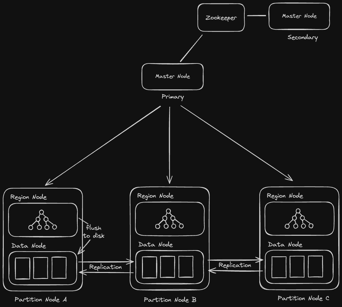
In addition to this, HBase also uses column oriented storage, which enables it to do large analytical queries and batch processing jobs over all the values for a single column efficiently.
When do we use HBase?
HBase is good if you want the flexibility of normal database operations over HDFS, as well as optimized batch processing. For most applications that require write optimization, Cassandra is probably better. However there are some use cases in which HBase may be a good choice - storing application logs for diagnostic and trend analysis, or storing clickstream data for downstream analysis, for exxample.
MapReduce is a programming model or pattern within the Hadoop framework that allows us to perform batch processing of big data sets. There are a few advantages to using MapReduce:
- We can run arbitrary code with custom mappers and reducers
- We can run computations on the same nodes that hold the data, granting us data locality benefits
- Failed mappers/reducers can be restarted independently
As the name implies, Mappers and Reducers are the basic building blocks of MapReduce:
- Mappers take an object and map it to a key-value pairing
- Reducers take a list of outputs produced by the mapper (over a single key) and reduce it to a single key-value pair
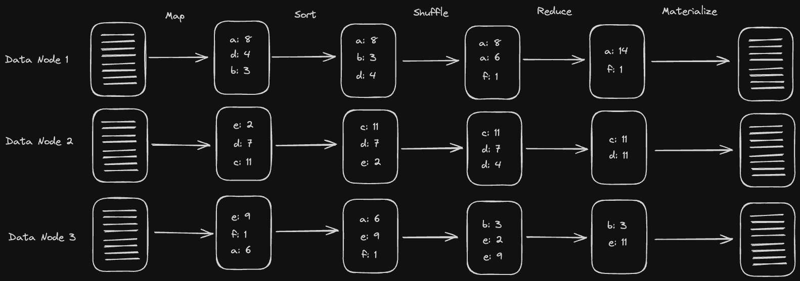
Every data node will have a bunch of unformatted data stored on disk. The MapReduce process then proceeds as follows (in memory on each data node):
- Map over all the data and turn it into key-value pairs using our Mappers
- Sort the keys. We'll explain why we do this later, but the gist is that it's easier to operate on sorted lists when we reduce.
- Shuffle the keys by hashing them and sending them to the node corresponding to the hash. This will ensure all the key-value pairs with the same key go to the same node. The sorted order of the keys is maintained on each node.
- Reduce the key-value pairs. We'll have a bunch of key-value pairs at this point that have the same key. We want to take all those and reduce it to just a single key-value pair for each key.
- Materialize the reduced data to disk
Here's a diagram of what that process might look like:
Why do we sort our keys?
During our reduce operation, if we have a sorted list of keys, we know that once we've seen the last key in the list, we can just flush the result to disk. Otherwise, we would have to store the intermediate result in memory in case we see another tuple for that key.
For example, assume we have the following data in our reducer and we'd like to compute the sum of values over each key:
Unsorted:
a: 6
a: 8
b: 3
<- At this point, we need to store the intermediate sum for "a" AND "b" in memory, since we might see more "a's" down the line
b: 7
a: 10
b: 4
Sorted:
a: 6
a: 8
a: 10
<- Once we've gotten here in our reducer, we can just flush the result for "a" to disk!
b: 3
b: 7
b: 4
Thus, sorting the data is much more memory efficient.
Job Chaining
Notice that every MapReduce job is just reading in data stored on disk for each data node, and then outputting it to data stored on disk at another or the same data node. Given that, we can actually just read in the outputs of one MapReduce as an input into another. This job chaining process allows us to achieve more complex functionality.
During batch computations, we might want to join multiple data sets together. For example, if we have some data like the following:
Favorite Websites:
---------------------
alice: "google.com"
alice: "facebook.com"
bob: "instagram.com"
bob: "reddit.com"

Age / Gender:
---------------------
alice: 22, Female
bob: 23, Male
We might want to produce the following joined result:
Favorite Websites with Age/Gender
---------------------------------
alice: "google.com", 22, Female
alice: "facebook.com", 22, Female
bob: "instagram.com", 23, Male
bob: "reddit.com", 23, Male
We have a few ways to do this:
Sort Merge Join
In a sort merge join, we sort the keys in each partition, then hash the keys to assign them to the same partition, and then join them together, effectively merging sorted lists
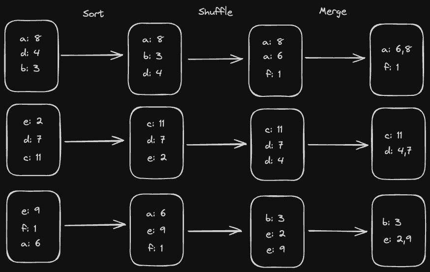
This can be slow since we need to sort all the data by the join key, and we’ll need to send at least one whole dataset over the network, possibly both depending on how they are partitioned
Broadcast Hash Join
If we have a small dataset, we can send it to all partitions and store them entirely in memory as a hash map. That's the basis for a Broadcast Hash Join, in which we linearly scan through our large dataset and check it against our hash map to join it.
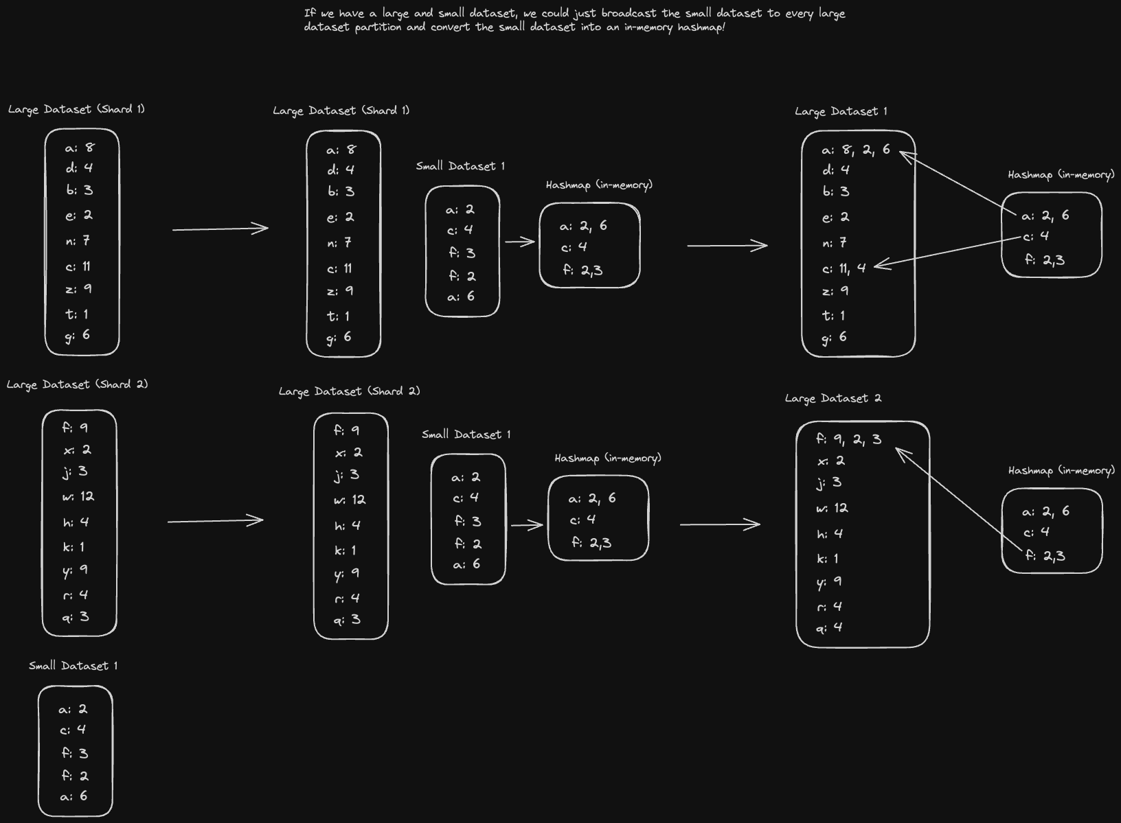
In this case, we don't need to sort our large dataset at all, saving a lot of time. Plus, sending just the small dataset over the network can be much more efficient.
Partition Hash Join
But what if neither dataset is small enough to fit in memory? That's where the partition hash join comes in - we can just partition the datasets into smaller datasets so that they do fit in memory. From there, we can just do a normal hash join.
It's important here that we partition both our datasets the same way so that the keys in each partition correspond to each other and go to the same node.
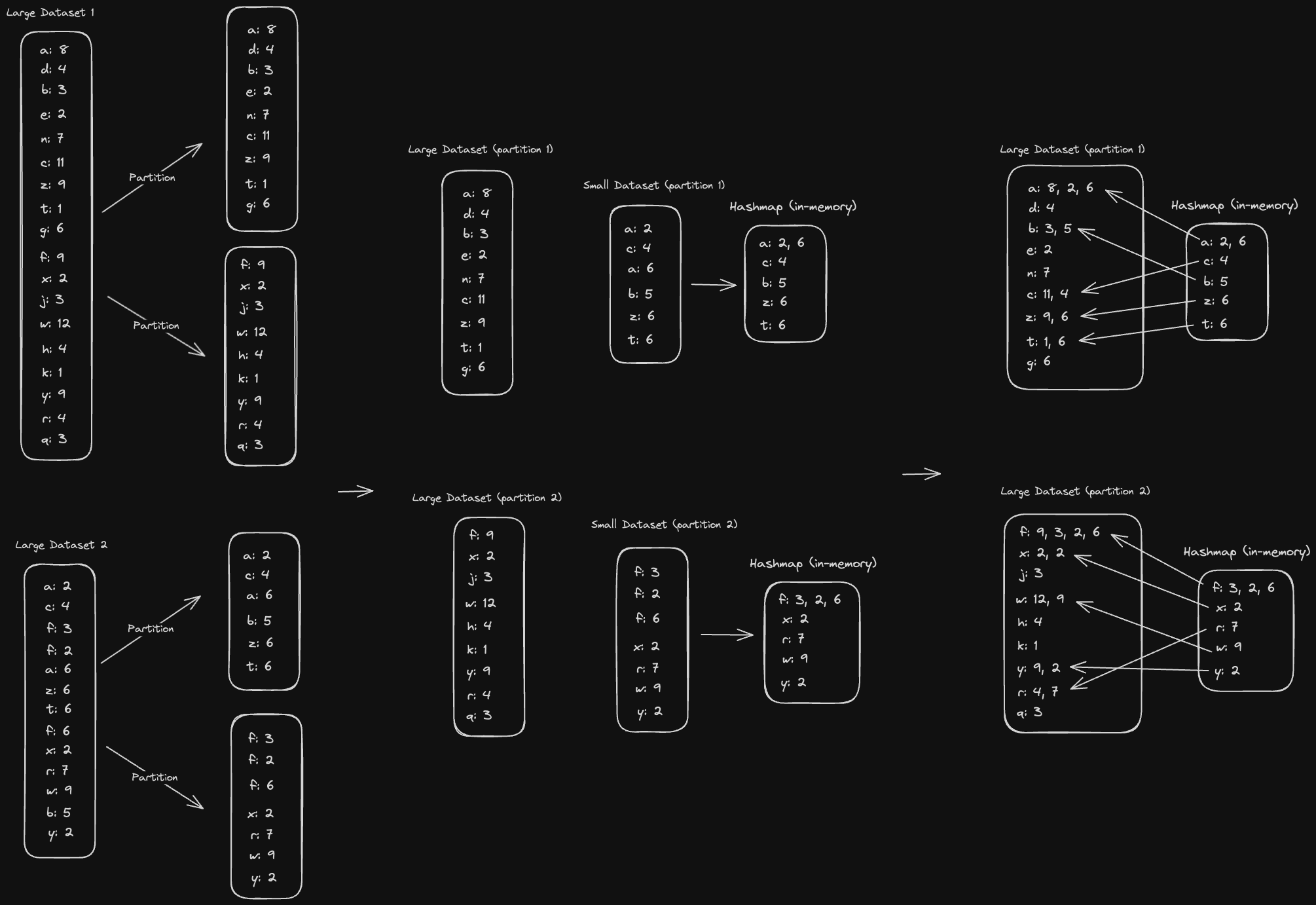
Though MapReduce is a nice framework for doing batch processing in HDFS, it isn't without its problems:
- Chained jobs in MapReduce are dependent on each other. If one takes a long time, it can block another from starting
- Each job requires a mapper and a reducer. Many times you won’t need more than one mapper, so if you have multiple jobs that all only really need 1 mapper you end up with a lot of unnecessary sorting
- Intermediate results of a MapReduce job are stored on disk, so we end up using a lot of disk space
Enter Apache Spark, which tries to address these issues:
- Nodes in Spark do computations as soon as possible instead of waiting for previous jobs to fully complete. As soon as it has all the data it needs, it proceeds to the next step
- Instead of requiring mappers and reducers, we instead have operator functions (which could be mapping or reducing)
- Spark stores intermediate states in memory instead of on disk. It only stores the input and output results on disk
Resilient Distributed Datasets (RDD)s are a core abstraction in Spark. They are immutable, distributed collections of elements of your data that can be operated on in parallel.
RDDs are abstractions of data collections sourced from multiple partitions and/or data stores (e.g. SQL tables, HDFS files, text files). Furthermore, Spark processes RDDs entirely in memory, which provides some nice performance benefits.
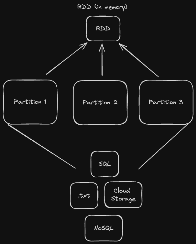
Spark applications are coordinated by a main program (known as a driver), which spins up a SparkContext object. The SparkContext object orchestrates tasks by talking to a cluster manager service like Kubernetes, Mesos, or Spark's own standalone cluster manager. It requests "executors" on nodes in the cluster, which are processes that perform computations and store data. The SparkContext then forwards application code (JAR or Python files) to the executors. Finally, it sends tasks to the cluster manager, which will then schedule and run them on the nodes using a Direct Acyclic Graph (DAG) Scheduler.
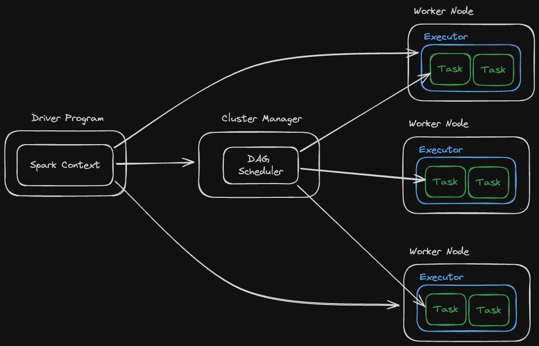
Of course, the fact that Spark does everything in memory naturally raises concerns about fault-tolerance. Fortunately, it has some mechanisms to ensure that we can recover from faults:
For narrow dependencies where computations on a given node don’t depend on data from other nodes, if a node goes down, its workload can be split across the remaining nodes and re-processed in parallel
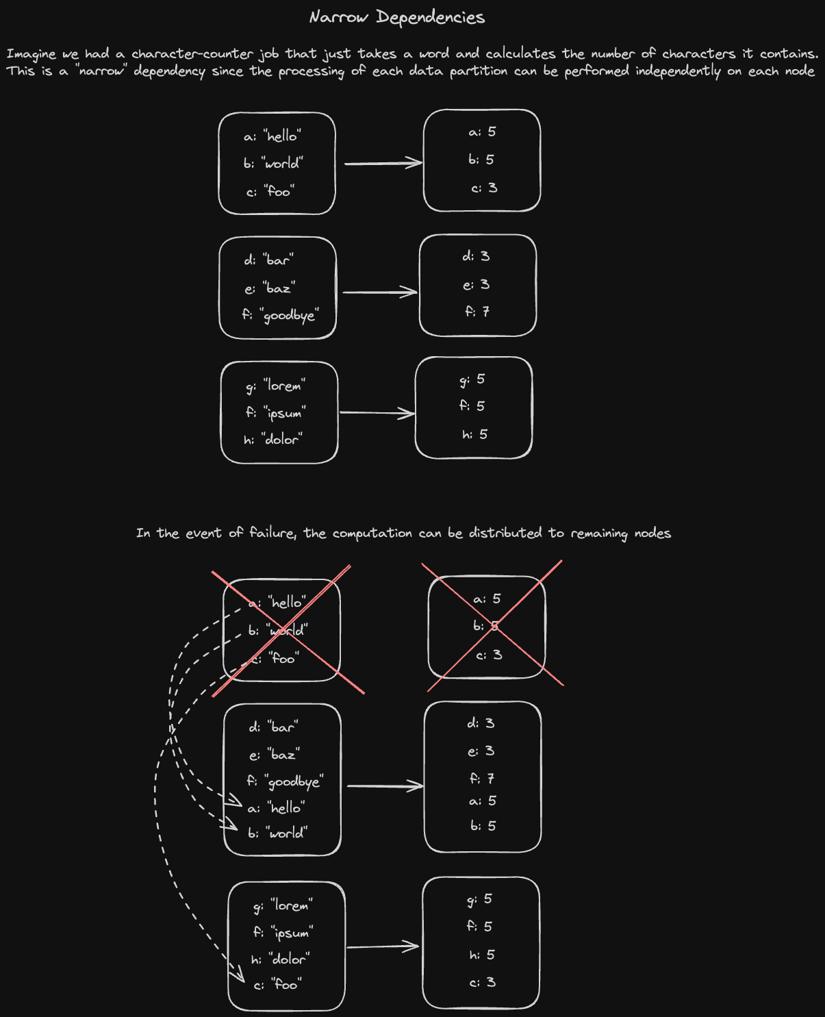
For wide dependencies where computations on a node depend on data from multiple other nodes, the process is much more tedious. If a node fails, its upstream states will need to be recomputed. Luckily, Spark automatically checkpoints data to disk after a wide dependency.
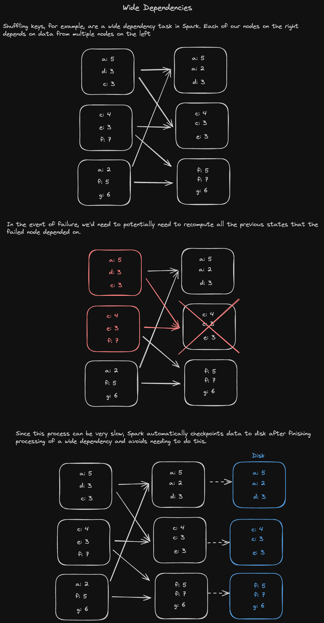
- Designing Data-Intensive Applications, Chapter 10, "Batch Processing"
- jordanhasnolife System Design 2.0 Playlist:
Unlike in batch processing, stream processing deals with unbounded data, or data that arrives gradually over time and is continually produced.
The general structure of stream processing systems involves two main stakeholders: producers and consumers. Producers, as the name implies, produce events. Consumers then consume those events.
Instead of having many long lived connections between producers and consumers to handle event propagation, we have a message broker, which takes on the responsibility of ingesting events from producers and pushing them to consumers. The typical underlying implementation of these are queues.
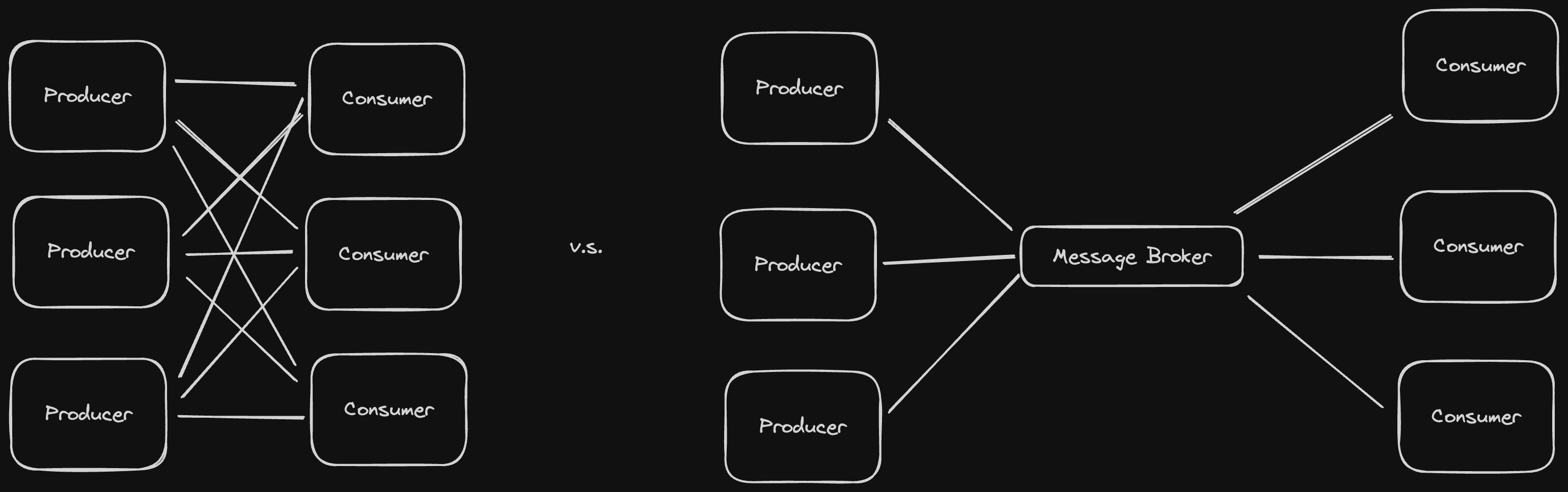
There are two types of message brokers: in-memory message brokers, and log-based message brokers
Examples: RabbitMQ, ActiveMQ, Azure Service Bus, Google Cloud Pub/Sub
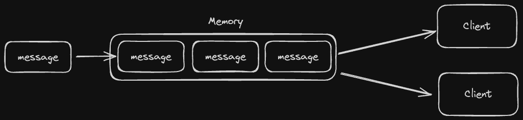
In-memory message brokers keep all messages in memory and typically optimize for higher throughput at the expense of ordered event processing and durability. Some typical use cases could include encoding user videos that get posted to Youtube, or sending user tweets to the news feeds of their followers
When a message gets delivered, it is marked for deletion from the queue. Once the consumer that received the message sends an ack that it was processed, the message is actually deleted. This could result in fault tolerance issues - if a message queue goes down, we don't have any way of replaying messages.
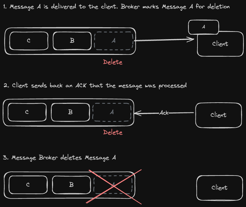
Messages are delivered to consumers in a round robin fashion. This means that if we have multiple consumers reading messages, they may not necessarily be processed in order. If the first consumer has a slow network connection or takes longer to process the message, the second consumer may end up finishing processing the subsequent message in the queue faster.
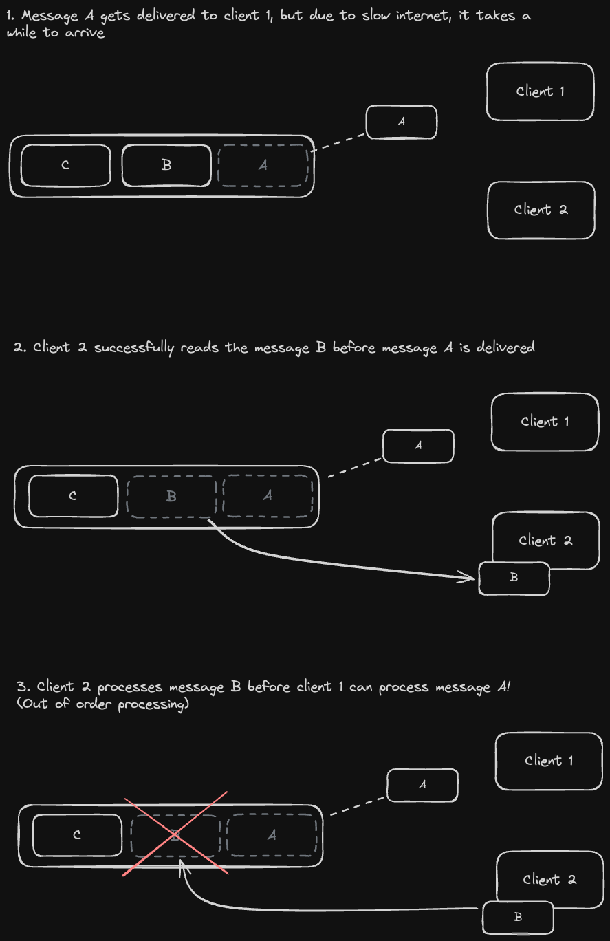
One way to avoid this is with fan out, where we partition our queue into multiple queues and have each consumer exclusively read from one queue. However, this would limit our throughput which kind of defeats the purpose of using an in-memory broker.
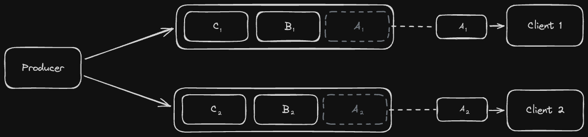
Examples: Apache Kafka, Amazon Kinesis Streams
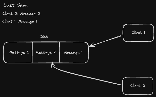
A log-based message broker keeps all its messages sequentially on disk and does not delete messages after they've been consumed. That inherently gives us more durability. Some use cases for these are processing a running average of sensor metrics, or doing change data capture - keeping writes from a database in sync with another derived data store.
Every message in a log-based message broker will be stored according to the order in which it arrived. Furthermore, log based brokers keep track of which messages consumers have seen to determine what message to send next. That means every message is processed in order, so one slow to process message could potentially slow down a consumer's overall read throughput. Of course, we could mitigate this with partitioning, similar to the fan out method in which other consumers read from other queues.
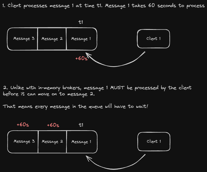
Exactly once message processing refers to the idea that we send a message both at least once and no more than once
At least once: In order to guarantee that a message is sent at least once, our message broker will need to be fault tolerant so that it can persist messages and resend in the event of failure. It will also need consumer acknowledgement that the message was received - if there are network issues and a message is not delivered successfully (lack of acknowledgement), the broker can retry.
No more than once: To ensure that a message is not sent more than once, we could use Two Phase Commit to perform a distributed transaction, guaranteeing that a consumer received and processed the message and then deleting it from the broker afterwards.
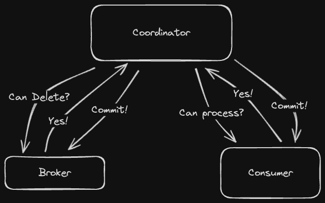
Otherwise, we could send the message multiple times but ensure that it isn't processed more than once. In other words, messages are idempotent - sending duplicates of the same message yields the same result as sending the message only once.
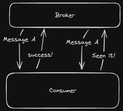
Here are a few common stream processing use cases:
Metric/Log Time Grouping and Bucketing
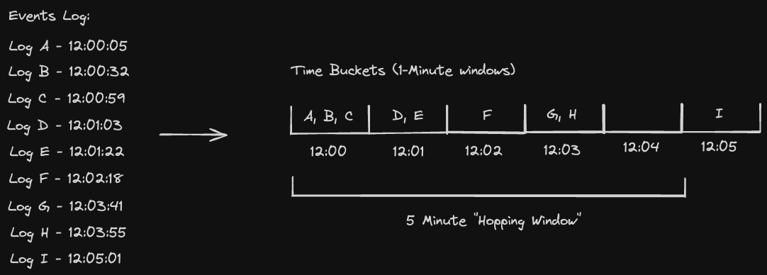
In Metric/Log time grouping and bucketing, we want to create time interval buckets (or "tumbling windows") and group events according to their timestamp
Sometimes we want to aggregate over many of these intervals in our analytics (hopping window). In this case, we can use a hashmap based on our time interval (for example, one minute), and group everything that occurs within that interval together.
Other times, we just want a sliding window (get me the events that occurred in the last 5 minutes). In this case, we can use a queue to track events as they arrive and evict old events that fall outside of our window
Change Data Capture
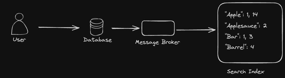
The idea behind Change Data Capture (CDC), is this: whenever we write to our database, we also want to store data derived from that change somewhere else (like a search index)
In practice, this means that writes to our database will publish an event to the message broker, which then updates the derived data store and keeps it in sync. This prevents us from needing to do two-phase commit between the database and the derived data store.
Event Sourcing
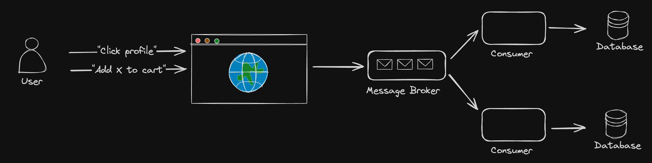
Event sourcing is similar to Change Data Capture, except that instead of writing to a database and then propagating those changes via a message broker to another data store, we write directly to the message broker itself.
The message broker can then surface events to any variety of consumers, which can then store them in a database.
An important thing to note is that events that get stored in message brokers are database agnostic, whereas in CDC data that's landing the message broker is database specific. This allows us to easily upgrade or switch out the databases that eventually store these events as long as we provide the translation logic to do so from our broker.
Event sourcing inherently assumes that the message broker is holding on to events. So that means we'd need a log-based message broker in order to facillitate this.
Stream enrichment is when we want to augment our stream events with more information and send them to other parts of our system. In other words, we want to join data from our streams with data from other sources (which themselves could be streams or databases) to produce some kind of aggregated or combined data.
In a stream-stream join, we want to join data from two streams together. For example, let's say we have two event producers: one for "Google Search Terms" and another for "Links clicked". We want to join events from the two so that we can correlate search terms with the resulting links that were clicked by a given user.
Since events from both producers might not come at the same time through our message broker, the consumer needs to cache events in memory, and match them with other events that correspond to the same key. In the example above, a user Alice may search the term "tissues", and the resulting link clicked event may not come until later. So the consumer would need to hold on to the { "Alice": tissues" } search term mapping until it sees the corresponding { "Alice": "amazon.com" } event and join the two.
In a stream table join, we now need to join events from a stream produce with data from a database. To use the previous example, let's say we had a "Demographics" table telling us the age and gender of our users. We want to join the "Google Search Terms" producer with our "Demographics" table.
A naive way to do this is to have our consumer query the database every time it receives a "Google Search Terms" event. This is inefficient since we'd need to perform a network request to the database every time.
We can do this more efficiently by storing an in-memory copy of our "Demographics" table in our consumer and using Change Data Capture to keep it in sync with the "Demographics" table in our database. In other words, we make a new write to the database, we propagate that change to our consumer using a message broker.
We can then use that in-memory table to perform the join whenever we receive an event from our "Google Search Terms" producer.
In a table-table join, we want to get join results as tables change. This is different from just a normal join, which is a static, one-shot operation.
To do this efficiently, we can use Change Data Capture in a similar fashion to our stream-table join example. We keep two in-memory copies of our tables in our consumer, and then perform CDC for each table to keep those in-memory tables in sync. Of course, two tables might be too big to fit in memory for one consumer. In that case, we'd need to partition our tables by the join key and perform CDC across multiple consumers.
As we saw in the previous join examples, we tend to need to keep state in memory in the consumer. As a result, we need a way to ensure fault tolerance in our consumers. Stream processing frameworks have mechanisms to ensure just that. Some examples of them include Flink, Spark Streaming, Tez, and Storm.
Note that all of these stream processing frameworks aren't the message queues, rather, they're the consumers.
Apache Flink is an open source, unified stream and batch processing framework. It allows us to have fault tolerance in our consumers and guarantees that each message only affect the state of each consumer once. An important caveat is that this guarantee only applies to consumers within the confines of our stream framework. We cannot guarantee that state outside of the framework will be affected only once when we replay messages after a crash.
Why is Fault Tolerance Hard?
Let's imagine a scenario where a consumer reads a message from queue A, performs some kind of stream join, and publishes the result to queue B. Before it's able to respond to queue A that it's successfully processed the message, it goes down. This means that queue A never moves to the next message in the queue, and so when the consumer comes back up, the same message will be processed and pushed to queue B again.
Flink Fault Tolerance
Flink solves this issue by saving checkpoints of each consumer on some form of durable storage (such as HDFS). These checkpoints contain the state of every consumer, so in the event of failures, the consumer states can be rebuilt from those checkpoints. Furthermore, since we're using log-based queues in these kinds of scenarios, Flink can replay the messages that occurred from our checkpoint onwards.
The way checkpoints are saved are via barrier messages. Flink designates a Job Manager node in our system that occasionally sends a barrier message through our queue, which, when received by a consumer, triggers a checkpoint to be created and saved.
These barrier messages propagate through all the consumers in our system, creating checkpoints that are causally consistent. Checkpoints for a consumer only get created if it recieves a barrier message from all of its upstream queues its reading from. Therefore, we are guaranteed that for a given checkpoint, all of the messages that have been processed by every consumer in our system are the same.
- Designing Data-Intensive Applications, Chapter 11, "Stream Processing"
- jordanhasnolife System Design 2.0 Playlist:
Sometimes, a traditional database or index isn't the optimal solution for certain situations (e.g. searching, tracking time series data, maintaining social graphs, or working with geographical data). This section will look at a variety of data stores and indexes for specialized use cases.
Database indexes aren’t very good for text searching because our search term might be any single substring of text stored in our DB
For example, a traditional index isn't going to help us search “Apple” in a dataset that contains “Apple”, “Cherry”, and “Green Apple” efficiently since "Cherry" comes before "Green Apple" lexicographically. Our index would return the ordering "Apple", "Cherry", and "Green Apple" when we want "Apple" and "Green Apple" to be next to each other
Search indices solve this problem using inverted indexes. Let's take a look at a few:
Prefix Inverted Index
In a prefix inverted index, we tokenize all the strings in our data and pair them with references to documents which contain those string tokens. To use our example from before, "Apple" would be a token, and the ids of documents containing "Apple" and "Green Apple" would be saved as references alongside that token.
Suffix Inverted Index
A suffix inverted index is essentially the same as prefix-inverted indexes, except we store reversed tokens. It allows us to easily search suffixes by using the reversed the suffix as our search term string and proceeding as normal
Apache Lucene is a popular open source search engine that supports complex text searches, Levenshtein distance, numerical searches, etc.
Elasticsearch is a convenience wrapper on top of Apache Lucene to allow for searching in a distributed system. It also provides some nice features out of the box:
- REST API
- Query language
- Managed replication and partitioning
- Visualization
- Uses local indexes per partition instead of a global index to reduce data duplication
- Generally wants to keep searches to one partition instead of aggregating search results across many partitions
- Smart caching
- Cache more common/frequently accessed parts of a query instead of the full query result or a piece of an index
A time series database is a database optimized for reading and writing time-series data. It uses column-oriented storage, which as we've seen previously, is better optimized for analytical queries over a single column.
Time series databases use hypertables to optimize reads and writes. A hypertable is a way to paramterize our data based on time and source. For example, we might have 3 sensors and 3 chunks of time (1-2PM, 2-3PM, 3-4PM). We can image a hypertable as being a 3x3 grid with sensors along the X-axis and time intervals along the Y-axis:
| Sensor 1 | Sensor2 | Sensor3 | |
|---|---|---|---|
| 1-2PM | |||
| 2-3PM | |||
| 3-4PM |
Each cell in the table above would correspond to a chunk of data for a given sensor between a given time interval.
Breaking data up in this way allows us to cache much more efficiently, since we can pinpoint with greater accuracy the exact data we want to load into our cache. It can allow us to optimize writes by enabling us to store these chunks in the same nodes as the sensors.
Finally, it can optimize deletes as well - since these databases typically also maintain an LSM Tree and SSTable, the traditional way to delete would be to write a tombstone to our LSM Tree and propagate that to disk. That means that deleting a bunch of data would incur the same cost as writing a bunch of data. With our chunk table, we don't need to do that - the organization of the data makes it easy to expire certain time interval chunks in disk by designating them as free memory that can just be overwritten.
- TimescaleDB - an open source, relational time series database
- InfluxDB - an open source time series database
- Apache Druid - a column oriented, open source distributed data store primarily used for Online Analytical Processing (OLAP) use cases
As the name implies, graph databases are used for representing graph data, or data that can be represented with vertices/nodes connected by edges
For instance, a social graph where the vertices are people and the edges represent some kind of relationship (friends with, following, is followed by, etc.)
Non-native graph databases take existing database implementations (like a relational database, for example), and provide a query language on top of it for graph traversals
In a relational database implementation, we'd have one table for vertices and another for edges
- Doing a graph traversal like querying all the neighbors of a given vertex would involve two separate binary searches on both the vertices and edges tables (assuming we have an index on both tables) - The time it takes to perform this query will grow as we add more vertices, so this is not ideal
In a non-relational database implementation, we could get rid of the edges table and just store the edges alongside with the vertex for better data locality
- To be more specific, a vertex would be represented as a JSON object with an
idand anedgeskey, which stores an array of all the vertex ids that are adjacent to this vertex - However, this would still require us to search the vertex table with all the vertex ids in the
edgesarray - Storing the full vertex in the
edgesarray is not viable since we'd have to store the neighboring vertices of those vertices in turn, and so on, creating a nested JSON abomination
Native graph databases, in contrast, are structured specifically to accomodate graph data
In Neo4J's implementation, we again have a vertex and edges table. However, this time each vertex row contains its own memory address, as well as the memory address of one of its edges
In turn, the edges table will have its own memory address, as well as the memory address of the vertex it points to. For a vertex that has multiple edges, the edge will also have the memory address of the next edge
It's akin to a linked list structure, where a vertex node will point to an edge node, and an edge node can point to another vertex node and another edge node
In the end, this means we don't have to perform binary searches on the vertices table whenever we want to find adjacent nodes. We can just follow the pointers and do it in constant time
Caveat: Random I/O on disk isn't great, but the time complexity savings compensate for this
Geospatial indexes specifically solve the problem of finding all points within some distance. For example, Doordash showing you the all the restaurants closest to you, or within some mile radius
Geohashes and quadtrees are the two key concepts that comprise a geospatial index.
A quadtree is a geographic plane split into 4 subplanes. These subplanes can then be recursively split into sub-quadtrees. A geohash is an address telling us which "leaf" subplane a particular point belongs to
- For example, if we have a plane broken into 4 subplanes A, B, C, D, and each subplane is recursively broken into sub-subplanes A, B, C, D, a geohash for a point could be "AB", telling us the point is stored a plane A, subplane B
- After determining the geohash of a point, we store these in sorted order (index) so that we can binary search them
The neat part is that the structure of our quadtrees makes it so that points that are lexicographically close to one another are also geographically close. Therefore, we can also use geohashes to partition data geographically, which is known as geosharding.
Big Data systems like Hadoop aren't great for storing static content because we’re not planning to run any compute over it, we generally just want to store and retrieve it later. In other words, we're wasting CPU resources when we want more disk space
An object store is a service offered by a cloud provider to store static content. They typically are managed services that handle scaling and replication and are schemaless; they're able to store any arbitrary file types
Data lakes, which are centralized repositories designed to store, process, and secure large amounts of structured, semi-structured, and unstructured data, are built on top of object stores since they typically stores data in its native format (blobs and files). Performing batch processing over this data would require us to export it to Hadoop for batch processing, which can be slow.
- 3.4 ElasticSearch Training - Inverted Index Explained
- jordanhasnolife System Design 2.0 Playlist:
In this section we'll take a look at some key concepts around computer networking, such as the protocols and mechanisms for transferring data between systems over a network or securing communications between client and server.
The OSI model is a logical and conceptual framework that divides network communications functions into seven layers. If you've ever heard the terms "L7" or "L4" with regards to networking, this is what that's referring to.
It encapsulates every type of network communication across both software and hardware components and ensures that two standalone systems can communicate via standardizd interfaces or protocols based on the current layer of operation.
The seven layers are as following:
- Physical - the physical cables and devices that deal with data transfer
- Data Link - the technologies used to connect two machines across a network where the physical layer exists (Ethernet, MAC)
- Network - concerned with routing, forwarding, and addressing across a dispersed network or multiple connected networks (IPv4, IPv6)
- Transport - focuses on ensuring data packets arrive in the right order without losses or errors and can recover seamlessly (TCP, UDP)
- Session - responsible for network coordination between two separate applications in a system (Network File System, or NFS, and Server Message Block, or SMB)
- Presentation - Concerned with the syntax of the data itself for applications to send and consume. (HTML, JSON)
- Application - Concerned with the specific type of application itself and its standardized communication methods (HTTPS, SMTP)
TCP, or Transmission Control Protocol, is a network protocol which provides reliable 2-way 1:1 communication through the use of handshakes and acknowledgements. TCP is used for most applications where reliability is crucial.
The process for establishing a connection is via a 3-way handshake:
- Send a SYN with a sequence number x
- Respond with an ACK with a sequence number x + 1 and a SYN with sequence number y
- Respond with ACK with a sequence number y + 1
TCP tries to guarantee reliable delivery using sequence numbers to confirm message receipt. This operates similarly to the handshake, send a message with a sequence number and expect an acknowledgment with the sequence number + 1
TCP also uses timeouts to retry whenever it doesn't receive an acknowledgement. For example, it sends a message with a sequence number, then waits for a set period before retrying the message. The amount of time it waits between retries increases exponentially; this is a strategy known as exponential backoff.
Flow control deals with ensuring that the sender isn't sending more messages than a receiver can consume. TCP does this by looking at the receiver buffer to limit the number of messages in flight. It then resets the limit upon receiving an acknowledgment.
Congestion control deals with ensuring that message traffic does not degrade network response times. TCP handles this by setting a window of how many messages can be sent at once. It then uses additive increase, multiplicative decrease (AIMD) to adjust the window size. AIMD dictates that the window should grow in size linearly when there's no congestion, but reduce in size exponentially when there is.
UDP, or User Datagram Protocol, is a simple, connectionless communication model without any of the reliability mechanisms that TCP provides. It's fairly bare bones - you just send packets from one node to another with some checksums for data integrity.
For that reason, it's super fast, and is used for low-latency scenarios where dropped data is acceptable. (e.g. video calls, video games, real-time tracking of stock prices). It also supports multicast, which is when a single packet is routed to multiple places.
Checksums are sent with every UDP header to ensure that packets aren't corrupted. Before sending off the segment, the sender:
- Computes the checksum based on the data in the segment
- Stores the computed checksum in the final two bytes of the UDP header
Upon receiving the data, the recipient
- Computes the checksum based on the received segment
- Compares it to the checksum in the header it received. If they aren't equal, it knows data was corrupted.
In traditional HTTP communication, the client sends requests to the server and waits for a response. Once received, the client needs to make a brand new requests to receive new data. This is "short polling", which might not be efficient for real time scenarios since we'd need to keep sending requests to the server.
Long Polling, on the other hand, keeps the requests open until new data is available. Once it receives that data, it completes the request and creates a new one. Since creating new connections is expensive, long polling is best used for situations where data is rarely needed. In addition, it's unidirectional, since data is only sent from the server to the client.
WebSocket is a communications protocol which provides persistent two-way communication between client and server. It's implemented over a single TCP connection, utilizes a special handshake incorporating the HTTP Upgrade Header to change from the HTTP protocol to WebSocket protocol, and has its own custom URI scheme: (ws:// for WebSocket) and (wss:// for Websocket Secure).
Since it's persistent, we avoid the overhead of creating new connections and dealing with request headers. However, if these connections are largely inactive, we might waste resources. In addition, if a connection goes down, the client will need to manually re-establish it.
Server-Sent Events provide a persistent, unidirectional communication channel that reconnects automatically.
Similar to Long Polling, communication is unidrectional from server to client. But then like with Websockets, we avoid the overhead of dealing with headers / time spent establishing connections since we create persistent connections. Of course, that also means we need to ensure we don't maintain too many inactive connections and waste resources
Automatic connection re-establishment is a convenient feature, however it might not necessarily be good. The thundering herd problem could occurr if the server goes down. When it comes back online it will try to re-establish connections with all the clients at once, causing a huge strain and potentially knocking it out again
A way to mitigate this is to use some random jitter similar to the leader candidate proposal process in the Raft distributed consensus algorithm.
TLS is a cryptographic protocol used to protect communications over a computer network. You probably know it as providing the "S" in "HTTPS". TLS ensures that data sent between clients and servers can't be eavesdropped on or tampered with.
TLS is typically thought of as "running on top of some reliable transport protocol", given that the name literally stands for "Transport layer Security". However, it's not a strictly L4 level protocol since it serves encryption to higher layers. Applications also need to actively initiate TLS handshakes and handle digital certificates.
When a client and server agree to use TLS, they use a handshake procedure to agree on the keys that they'll both use to encrypt/decrypt their data. The handshake goes like this:
-
A client connects to a TLS enabled server and presents a list of supported cipher suites and hash functions. These include algorithms for exchanging keys, encrypting data, and verifying data integrity.
-
The server picks a cipher and hash function and notifies the client
-
The server then provides identification in the form of a digital certificate. The certificate contains the server name, trusted certificate authority that vouches for its authenticity, and a public encryption key.
-
The client confirms the validity of the certificate
-
The client and server now generate session keys in one of two ways:
a. The client encrypts a random number with the server's public encryption key, which the server then decrypts with its private key. Both then use this random number to generate a unique session key for subsequent encryption/decryption.
b. The client and server use the Diffie-Helman key exchange algorithm to securely generate a random and unique session key. This gives us the nice benefit of ensuring that the session cannot be decrypted even if the private key leaks on the server, which is known as forward secrecy
Performing this key exchange and subsequent encryption/decryption of data can be CPU intensive on our application servers. A common pattern to mitigate this is to terminate TLS using a proxy server (like a load balancer), and use regular HTTP when communicating between servers internally in our system.
Doing this comes with all the added complexity of managing proxy load-balancer servers - we'd want to do this in a fault-tolerant way and without bottlenecking our system, which we talk about a bit more in the load balancers section. Furthermore, if the proxy is compromised, then all our data throughout our system is available since it's unencrypted.
The Domain Name System is responsible for turning domain names (like www.google.com) into IP addresses that computers can understand. It has two main components: DNS resolvers and DNS name servers, which work in a hierarchical, distributed fashion to resolve queries in a robust and performant manner.
Let's take a deeper look:
The DNS resolver is a server that's responsible for sending and coordinating further downstream requests to DNS nameservers. Resolvers are maintained by ISPs and popular DNS providers like Google (8.8.8.8) and CloudFlare (1.1.1.1).
DNS Nameservers are servers that are responsible for locating the domain's corresponding IP in a hierarchical fashion. There are 3 types of nameservers
-
Root Nameservers: the first server that the DNS resolver reaches out to, which mainly just stores the IP addresses of the TLD nameservers.
-
TLD (Top Level Domain) Nameserver: the next level of our nameserver hierarchy, which typically hosts the last portion of a given domain (.com, .net, .org) and stores the IP addresses of the respective authoritative nameservers.
-
Authoritative Nameserver: the final level of the hierarchy which provides an authoritative answer for a given domain query. This is where the full domain name mapping record is stored (e.g. google.com, amazon.com).
Let's take a look at an example where a user types "www.google.com" into their browser.
-
First, the browser checks its cache. If the result isn't there, it makes an operating system call which checks its cache and reaches out to the DNS resolver.
-
If the result isn't cached at the DNS resolver level, the resolver reaches out to the Root Nameserver, which responds with a list of ".com" TLD nameserver IP addresses.
-
The DNS Resolver then reaches out to one of these ".com" TLD nameservers, which returns the IP address for the "google.com" authoritative nameserver.
-
Finally, the DNS Resolver gets the IP address for "google.com" from the authoritative nameserver and returns the result to the OS, which can then return that result to the browser.
When we register a new domain or change a domain record, we need to wait for it to propagate across all the DNS nameservers. This can be slow since nameservers cache domain record information for a certain amount of time (TTL) before refreshing. Since these TTLs are configured on the records themselves, one way we can speed up DNS propagation is to decrease the TTL value one day before implementing a change.
There are various online tools for checking if DNS record changes have propagated globally, such as Global DNS Checker or Google's DNS Checker.
- KhanAcademy "Computers and the Internet: User Datagram Protocol"
- PubNub "What is Long Polling?"
- AWS Cloud Computing Concepts Hub "What is OSI Model?"
- jordanhasnolife System Design 2.0 Playlist:
- Hussein Nasser: "SSL/TLS Termination, TLS Forward Proxy Pros and Cons"
- ByteByteGo: "Everything You Need To Know About DNS"
- CloudFlare Learning Center: "What is DNS | How DNS works"
Load balancing is the method of distributing network traffic equally across a pool of resources that support an application. It's very important in a distributed system to load balance intelligently so we don't overwhelm any of our key components whenever we have large amounts of traffic coming through.
First, let's look at the different ways we can scale a system
Vertical scaling means improving the performance of our system by upgrading the hardware of our application server or database node.
Horizontal scaling means improving performance by distributing computational load across more machines, which are usually commodity hardware. This is typically where load balancing comes into play
There are several ways to route traffic in our load balancers:
Weighted or Unweighted Round Robin:
A round robin policy is when we distribute requests to each server sequentially and wrap around. (you can imagine it's like dealing cards in Poker to each player).
An unweighted round robin strategy just means we naively distribute traffic equally across all our nodes. In constrast, a weighted strategy sends more requests to a given node if it has a greater weight.
Lowest Response Time:
In a lowest response time routing strategy, we keep a running average of the response times of each node. We then route requests to the ones with the lowest response time.
Hashing:
Hashing is where we take a hash of request content or headers and distribute load to each node corresponding to the hash value. We can do this at the L4 or L7 layer. (Recall in the OSI model of networking, L4 corresponds to the Transport Layer, like TCP, and L7 corresponds to the application layer, like HTTP)
- L4: Hash information based on information exposed at the networking layer, like IP, protocol, etc. (faster).
- L7: Hash information available in the actual message content (slower but more flexible).
It's important that we use consistent hashing so that every request goes to the same partition.
Let's look at 2 ways we can ensure fault tolerance in our load balancer setups.
In an active-active setup, we have more than 1 active load balancer. That means requests come into both load balancers, and both load balancers actively redirect traffic to the appropriate downstream application servers.
Pros
- Higher throughput since requests can be split across the two load balancers.
- Fault tolerance since we essentially have replicas of our load balancers.
Cons
- Might make local state maintained on the load balancer (like keeping track of average response time per server) a bit more complicated.
- Complexity in configuration.
- Potentially higher costs since we need to run multiple load balancers at full capacity.
In an active-passive setup, we have an active load balancer that actually performs the request routing and one passive one that sits idly on standby. We utilize a coordinator service like Zookeeper, which will continuously send heartbeats to the active load balancer and swap over to the passive one in the event of a failure.
Pros:
- Simplicity - we just have one load balancer to manage.
- Cost-effective - only one load balancer is run at full capacity.
Cons:
- Lower throughput.
- Underutilization of resources in passive nodes.
jordanhasnolife System Design 2.0 Playlist "Load Balancing - The Right Way to Do It"
In this section, we'll take a look at how software systems are typically organized at scale and the tradeoffs associated with various paradigms.
A Monolithic architecture is a singular system with one code base that couples all business concerns together. These are convenient early on in a project's life since they're easy to understand and manage. Testing and debugging is streamlined since we just have a single codebase or service, and we don't need to coordinate business logic across multiple endpoints which might give us some nice performance benefits.
However as a system grows, some major problems begin to arise: For one thing, we have a single point of failure so our system is less reliable. We also can't scale up individual parts of our system independently, or use different technologies for each part since it's one giant codebase. Finally, making changes requires updating and deploying the entire system, which can be slow and inefficient.
A Microservices architecture relies on coordinating a series of independently managed and deployed services. Each "microservice" is responsible for doing one thing and thus all development and testing is encapsulated. They solve for many of the problems we saw before with monolithic architectures in that they allow for faster, smaller scale updates to our system and the flexibility to choose different technologies which might be more suited for specific domains. They also give us higher reliability - we can isolate failures within our system now that logic is split across many different services.
There are some downsides as well - with more services comes more management complexity and costs. Communication and agreement on interfaces across service owner teams can bog down development speed. Allowing a variety of technologies can degrade standardization and present challenges in logging and monitoring. Furthermore, with each new service comes its own hosting infrastructure and tooling, which could mean exponentially increasing costs as the system scales.
Microservices architectures are widely adopted at large companies operating at high scale, so the next few sections will explore some methods of developing and maintaining them.
A container is a standard unit of software that packages up code and all its dependencies for reliable, efficient execution and deployment. In the context of microservices, each service might be using different technologies and runtimes. Containers allow us to bundle these up in a nice, scalable way.
A widely used platform for building and maintaing software containers is Docker
Virtual Machines are instances of operating systems co-located on the same physical machine. These are coordinated through the use of a hypervisor, which abstracts the physical host hardware from the operating system environment. Each Virtual Machine has its own OS, memory and other resources, which are isolated from other VMs.
Containers, on the other hand, are lightweight, portable, executable images that only concern themselves with application software and their dependencies. Unlike VMs, they share the same operating system kernel so they use fewer resources and can start and stop faster. Containers also allow us to dynamically scale resources, unlike VMs, where we need to specify our resource requirements in advance.
Virtual Machines and containers aren't mutually exclusive. A container could run within a VM to reap the benefits of both worlds, namely the portability and speed afforded by containers and the security afforded by isolated VM environments.
A few problems arise when we start using a whole bunch of containers together in our microservices architecture. How do we know which host to put each container on? And what should we do in the event of a host failure?
Kubernetes and other container management systems provide a "control plane" to deal with these kinds of issues. In Kubernetes specifically, we have a control plane node that runs some kind of coordination service like Zookeeper or Etcd. It talks to all of our hosts through "Kubelets", which are agents that run on each host. These Kubelets coordinate and provision "pods", which correspond to individual Docker containers. If a container fails, the Kubelet can restart it, and if a host goes down, the control plane can replicate it over to another host.
In previous sections, we looked a the microservices architecture and the advantages it gives us in terms of independent scalability, flexibility, and reliability in a large software system. If you'll recall, one of the drawbacks was the inability to enforce standardized monitoring and logging across these hundreds or potentially thousands of services.
Enter the ELK stack - an acronym used to describe a technology stack comprised of three popular technologies, Elasticsearch, Logstash, and Kibana. The ELK stack aims to provide an easy way to aggregate, analyze and vizualize logs across many different services, and has become very popular for troubleshooting and monitoring large microservices-based systems.
Let's take a look at each component in further detail
We briefly mentioned Elasticsearch we we talked about search indexes. As a refresher, it's a distributed search index built on top of Apache Lucene, and it provides some nice features for analytics and querying. The key thing to note in the context of the ELK stack is that often times, Elasticsearch is used more as a datastore for logs than as a search index
Logstash is an open source data-ingestion tool that transforms and aggregates data from multiple sources to be republished elswhere. It functions as the entrypoint for your microservices to send their logs to. Traditionally it was used to just parse and forward log data to Elasticsearch to be analyzed. In more recent years, Logstash has started to become a more general-purpose stream processing consumer, and has a rich plugin ecosystem that lets you customize how you ingest, parse, and publish your data, with support for multiple downstream destinations (which it refers to as "stashes").
Kibana is an analytics and visualization platform which serves as the view layer for the ELK stack. It provides rich functionality for creating various realtime data visualizations like charts, maps and tables. It's basically a web platform that queries data from Elasticsearch via its REST API and provides configurations for how to display the results.
Today, the ELK Stack has evolved to incorporate two new components (X-Pack and Beats) and is now more commonly referred to as the "Elastic stack". X-Pack is a pack of features which provide additional functionality on top of ElasticSearch, such as graph visualizations and machine learning based anomaly detection. Beats is an event publishing agent that can be installed on your microservice hosts to standardize how you publish your log files (FileBeat) and metrics (MetricBeat).
Note: The ELK stack started off as a fully open source project, but has recently become a proprietary, managed offering provided by the Elastic NV company after transitioning from the Apache License v2 to the dual Server Side Public License and Elastic License. AWS provides alternatives to Elasticsearch and Kibana under the old Apache License in the form of OpenSearch and OpenSearch Dashboards.
Fault tolerance becomes a non-trivial problem when we have hundreds of microservices interacting with each other. What happens when a critical service with lots of upstream dependencies fails? A typical way to recover from failures is to retry the requests, and exponentially back off (similar to the way TCP performs congestion control). However, if the service is down for an extended period of time, we could end up with retried requests piling up in these upstream dependencies, leading to resource exhaustion and cascading failures.
The circuit breaker patern aims to solve the problem of cascading failures as a result of service downtime. As the name implies, the circuit breaker pattern is based on electrical circuit breakers, which automatically interrupt current flow during power surges or faults to protect cascading failures in your electronic devices and appliances.
Software circuit breakers are practically implemented as request interceptors and have 3 states: open, half open, and closed:
- When the circuit breaker is closed, it allows requests to execute normally. While doing so, it measures faults and successes, and if the number of faults exceed a certain threshold, the circuit will break and enter the open state.
- When the circuit breaker is open, it prevents the execution of all requests passing through it. The circuit breaker will remain in this state for some configured timespan, at which point it will enter the half-open state.
- Finally, when the circuit breaker is half-open, it will retry some but not all of the failed requests. If these requests continue to fail, the circuit breaker will re-enter the open state and remain that way for another break period. Otherwise, it will close and start handling requests normally.
One additional optimization we can make is to configure a fallback policy. When a downstream API fails, we can specify an alternative backup service or cache that the circuit breaker can redirect requests to. This will give us higher availability in our overall system, as we can continue to satisfy client queries when a service breaks.
Another way to provide fault tolerance is to pre-emptively rate-limit upstream dependencies from flooding our service with requests. This is especially important when we're dealing with malicious threats to fault tolerance external to our system, such as Distributed Denial of Service (DDOS) attacks.
There are a few ways of rate-limiting and API throttling in software systems:
-
Fixed Window: Specifiy a limit on how many requests a client can send in a fixed window of time. After the fixed window passes, that limit resets.
-
Token Bucket: We specify a "bucket" with a capacity to hold N tokens. Whenever a request comes in, it "redeems" a token and is fulfilled. When all the tokens are gone, requests will be dropped / fail. The bucket will refill tokens at some speficied maximum refill rate.
- The maximum refill rate in this scenario is the maximum rate that users will have on average.
- The max capacity can be larger than the max refill rate. That means that for a given point in time, we could have a large number of requests coming in at once which consumes all available tokens (capacity). However subsequent requests will need to wait for the tokens to refill. Thus we are able to accommodate bursty traffic while still guaranteeing a maximum requests per second rate.
- Hystrix was a latency and fault tolerance library designed by Netflix to isolate points of access to remote systems, services and 3rd party libraries. It entered maintenance mode in 2020.
- Resilience4J has been the replacement for Hystrix ever since, and is a lightweight fault tolerance library with a functional programming model for Java applications. It implements the circuit breaker, rate-limiter, and retry patterns
Serverless computing is a method of providing compute resources on an as-used basis, enabling users to write and deploy code without needing to worry about the underlying infrastructure. The concept was first pioneered by Amazon in 2014 with the introduction of AWS Lambda.
The term serverless is somewhat of a misnomer, as servers are still being used behind the scenes. The main selling point is that the actual configuration and provisioning of those servers is entirely handled by the vendor, effectively hiding them from the developer.
Some examples of serverless providers (other than AWS Lambda) are:
Serverless computing has several advantages:
- Potentially lower cost: If services have uneven traffic load, serverless may be a more cost-effective solution since we don't waste resources and money running idle servers
- Simplified scalability: Vendors automatically scale resource allocation based on usage, vastly simplifying the process for developers.
- Simplified code: Typically the developer just writes a function rather than needing to setup all the boilerplate for running a server.
However, it has some downsides:
-
Cold Start Problem: When serverless functions aren't invoked for a long time, vendors will dynamically scale down resource usage to zero. Subsequent invocations to this "cold" function will require all of these resources to be spun back up, which could result in high latency
- There are some ways of mitigating this, such as a minimum allocation setting to keep functions "warm"
-
Costly for multi-step workflows or long-running processes: Long running processes with consistent load are typically better off using traditional servers. Reserved hardware is typically much more cost effective in these scenarios.
Furthermore, multi-step workflows can be extremely inefficient and expensive. A famous example is when Amazon Prime Video cut costs by 90% in 2023 after switching from a serverless architecture to a monolithic one for their video-quality inspection workflow.
- Atlassian Microservices Guide: "Monolithic vs. Microservices Architecture"
- jordanhasnolife System Design 2.0: "Monolith vs. Microservices + Docker + Kubernetes"
- Google Cloud: "Containers vs. VMs"
- Coding Explained: "Overview of the Elastic Stack (formerly ELK Stack)"
- AWS Cloud Computing Concepts Hub: "What is the ELK Stack?"
- Nick Chapsas: "The Circuit Breaker Pattern | Resilient Microservices"
- Be A Better Dev: "What is Rate Limiting / API Throttling? | System Design Concepts"
- Cloudflare Learning Center: "What is Serverless?"