nssvie

A python package for computing a numerical solution of stochastic Volterra integral equations of the second kind

where

• is an unknown process,
• is a continuous function,
• are continuous and square integrable functions,
• is the Brownian motion (see Wiener process) and
• is the Itô-integral (see Itô calculus)

by a stochastic operational matrix based on block pulse functions as suggested in Maleknejad et. al (2012)¹.

• Documentation
• API Reference
• Source Code
• Bug reports

nssvie is distributed under the terms of the GNU GPLv3 license.

Install

Install using either of the following two methods.

1. Install from PyPi

The nssvie package is available on PyPi and can be installed using pip

pip install nssvie

2. Install from Source

Install directly from the source code by

git clone https://github.com/dsagolla/nssvie.git
cd nssvie
pip install .   

Dependencies

nssvie uses

• NumPy for many calculations,
• SciPy for computing the block pulse coefficients and
• stochastic for sampling the Brownian Motion

Usage

Consider the following example of a stochastic Volterra integral equation

so

• ,
• and
• .

from nssvie import SVIE
import matplotlib.pyplot as plt

# Define the function and the kernels of the stochastic Volterra 
# integral equation
def f(t):
    return 1.0

def k1(s,t):
    return s**2

def k2(s,t):
    return s

# Generate the stochastic Volterra integral equation
svie = SVIE(
    function_f=f, kernel_2=k1, kernel_1=k2, endpoint=0.5
)
# Calculate numerical solution with m=20 intervals  
approximative_solution = svie.solve_numerical(
    intervals=20
)
fig, ax = plt.subplots()
times = [i * 0.5/20 for i in range(21)]
ax.step(times, approximative_solution, c='k')
plt.show()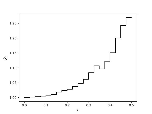

The parameters are

• function_f: the function .
• kernel_1, kernel_2: the kernels .
• endpoint: the right hand side of [0, T) (default is 1.0),
• intervals: the number of intervals to divide [0, T) (default is 50)

for the stochastic Volterra integral equation above.

Citation

---

1. Maleknejad, K., Khodabin, M., & Rostami, M. (2012). Numerical solution of stochastic Volterra integral equations by a stochastic operational matrix based on block pulse functions. Mathematical and computer Modelling, 55(3-4), 791-800. ↩