Computer Vision Model
The following sections describe the computer vision model and current results in more detail.
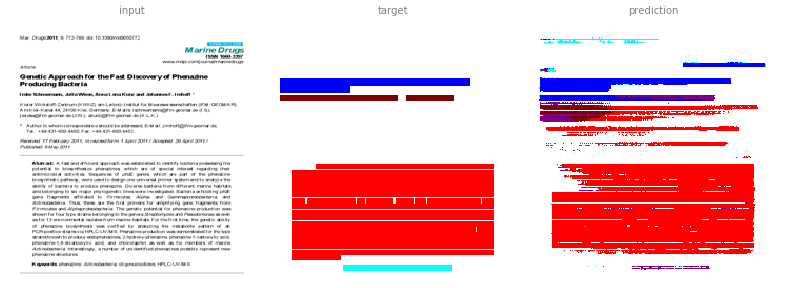
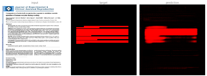
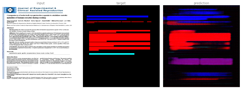
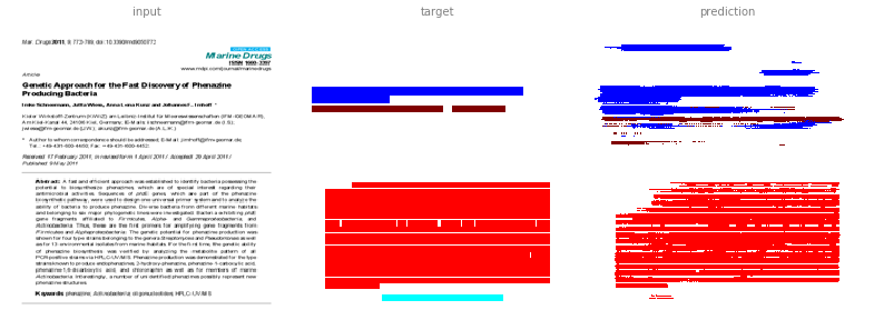
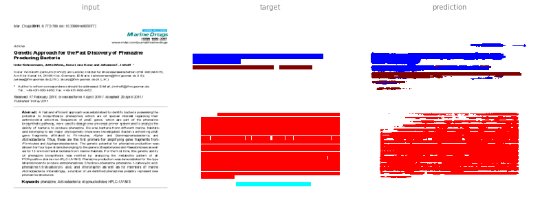
For the computer vision task, we've prepared an image of the PDF page, as well as the annotated areas.
From the input (image of PDF page):

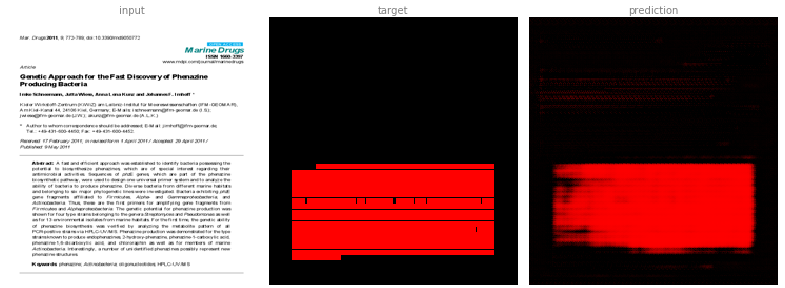
This image is a derivative of and attributed to Schneemann, I.; Wiese, J.; Kunz, A.L.; Imhoff, J.F. Genetic Approach for the Fast Discovery of Phenazine Producing Bacteria. Mar. Drugs 2011, 9, 772-789, and used under CC BY 3.0.
We expect the model to learn the 'annotated' image:
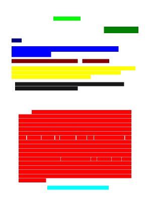
That is problem is typically referred to as 'semantic segmentation' (or sometimes just image segmentation).
So far we have used the PMC_sample_1943 dataset, containing one manuscript for each of the 1943 different journals in the dataset. A copy is available from the GROBID End-to-end evaluation.
We have trained the model on 900 of those manuscripts and tested the model on other manuscripts of the same dataset.
For the purpose of this model we treated section paragraphs (with section title) and main paragraphs (without section title) the same.
These are PDFs from publishers, i.e. been through production, so are more structured already than author versions. Good to start training model on these as well-structured and we have the publisher’s XML. Ultimately, for pipeline to be useful for converting author PDFs, such as on preprint server, into XML for text mining, we will need to continue to train the model on author-submitted PDFs. These have more variety in their structure, plus the accompanying metadata are more variable. First, we need a good model from the best data we have (publisher side).
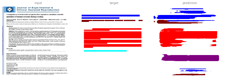
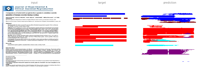
The model is currently based on the pix2pix model (and it's TensorFlow Model).
Treating the annotation as a regular RGB image, we already get fairly good results on first samples:
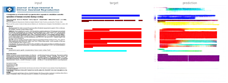
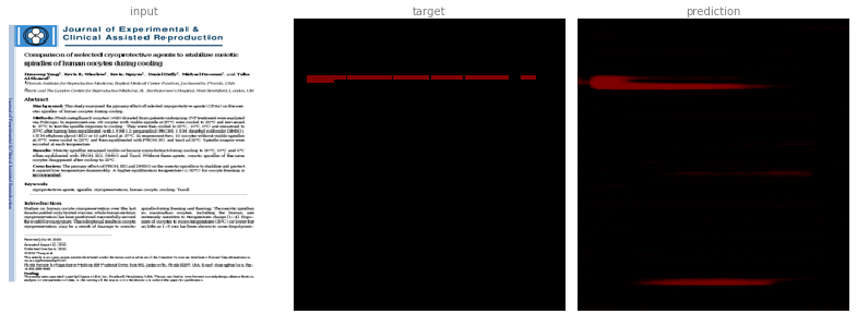
This image is a derivative of and attributed to Yang D, Winslow KL, Nguyen K, Duffy D, Freeman M, Al-Shawaf T. Comparison of selected cryoprotective agents to stabilize meiotic spindles of human oocytes during cooling. Journal of Experimental & Clinical Assisted Reproduction. 2010;7:4, and used under CC BY 2.0.
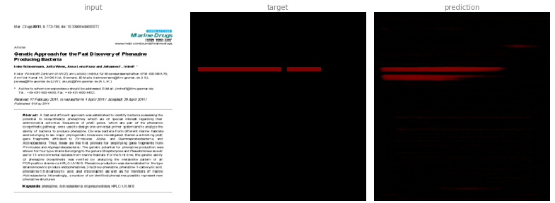
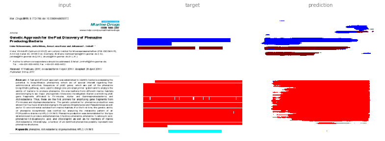
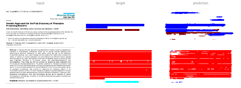
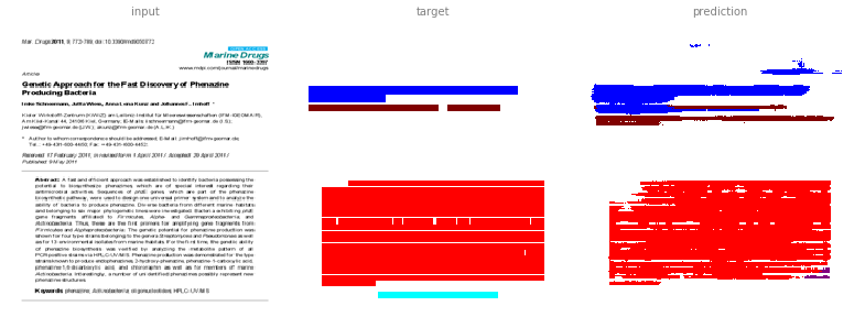
This image is a derivative of and attributed to Schneemann, I.; Wiese, J.; Kunz, A.L.; Imhoff, J.F. Genetic Approach for the Fast Discovery of Phenazine Producing Bacteria. Mar. Drugs 2011, 9, 772-789, and used under CC BY 3.0.
The results are not perfect but still promising. In the first example it learned to annotate paragraphs (purple) that were incorrectly absent from the test annotation.
To find the manuscript title, we would look for the blue coloured area.
Since the colours do not match exactly, we are first finding the closest colour as illustrated for the first example.
One issue we might encounter is that the blue (and other colours) will be shaded and sometimes mix with other colours.
But while mixing red (abstract) and blue (manuscript title) would result in purple (paragraph), that relationship doesn’t make any sense for the annotation (abstract + manuscript title != paragraph) itself.
To address this issue, we could use separate output channels.
For example we could assign the R, G, B channels each a class, as follows: red for abstract, green for doi (identifier), and blue for title.

The alternative is to use more channels, and assign each channel to a specific tag.
The model itself is not limited to RGB but can also handle say 20 channels.
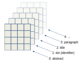
Initially we selected the following layers to focus on:
abstractauthorkeywordsmanuscript titlesection paragraph
We also added another layer for unknown (or none) class. That will help us to find the highest probability, including the background.
In preliminary tests comparing this multi-channel method against the RGB method, it is not clear which method is preferable. But using separate channels allows us to get probabilities out of the model.
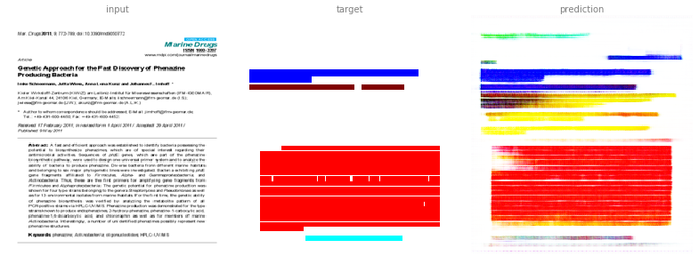
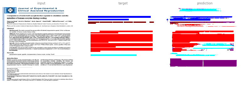
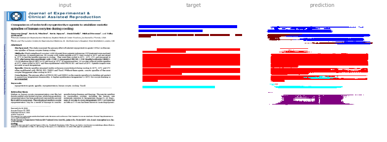
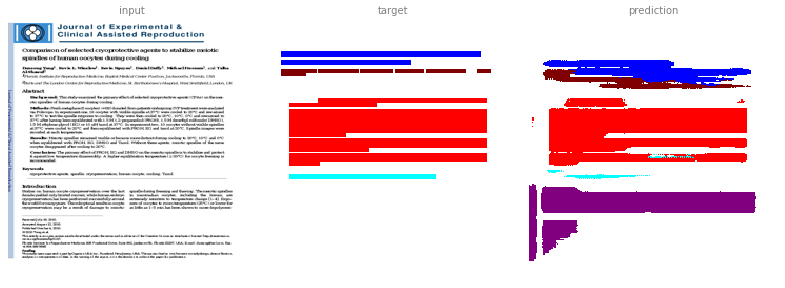
The multi-channel method has been able to learn the manuscript title block fairly well, here coloured in blue, for this first sample, but it is predicting a larger area than is accurate for the second sample.
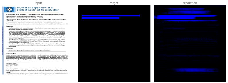
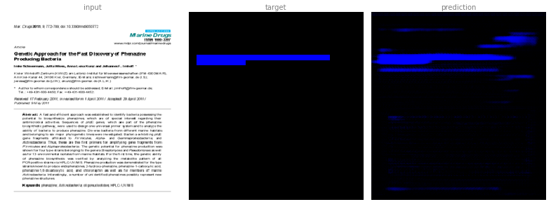
In the case of the abstract channel, here identified with red, we can see that the multi-channel method still wrongly identifies the first paragraph in sample two as an abstract, as it did for the RGB method too.
The author channel also proves difficult. In this case, the RGB method was better than the multi-channel method. It may be that we need to use a higher resolution input image.
Combining all the channels together gives us a general overview. This image isn’t useful for further processing, however, as individual channels are required to identify separately tagged blocks.

What we might want to do, if we don't need the probabilities, is to select the colour with the highest probability. This is also where the unknown layer (in white) comes in handy as it should have the highest probability where no other class is annotated.
At this point the output became distinct classes and the problem should be treated as a (multiclass classification)[https://en.wikipedia.org/wiki/Multiclass_classification]. The default loss used so far has been L1. We are going to use softmax + cross entropy.
Visually the improvement may not be clear. The quantitative scores are noticably better though.
One extention to the previous steps is to make to have separate discriminator outputs per channel. That can for example be achieved by creating separate discriminators per channel.
Quantitative the results are not much different. The computation became significant more expensive (in terms of memory and time - it took about 3x as long to train). That approach will get more expensive the more classes we train.
We also tried a using multiple discriminators with shared weights but multiple output channels. Not surprisingly with very similar quantitative results but less expensive (it took about 2x as long to train).
Another alternative would be to use a discriminator with the channel as a conditional. But other than efficiency it would unlikely improve the results.
We also contrasted it with the no discriminator at all (i.e. not using GAN).

The results are quantitatively also very similar, which seem to indicate that we don't benefit much from the GAN architecture in this case. Which would be consistent with the original pix2pix paper. But a similar approach had been found to improve the result in more recent work (SegAN and Semi and Weakly Supervised GAN).
Some indicative results:
The F1 score for the pixel wise match as a unweighted multi class classification.
Limited to the following classes:
abstractauthorkeywordsmanuscript titlesection paragraph
Over 400 test samples.
Note: The results are only indicative. More needs to be done to make those numbers reliable (e.g. multiple runs, etc.).
Improve the model further, some ideas:
- allow model to use the structure / hierachy:
- the model already has access to the hierachy but may be limited
- add extra layer(s) or CRF
- explore semi-supervised GAN architecture:
- currently the generator is the main output, improved by the discriminator
- explore the use of a GAN architecture that learns to generates training data
- explore other ways to generate training data
- explore reinforcement learning?
- allow the model to learn for longer (currently it has been limited to 1000 steps)
(some of those suggestions were made at a recent TensorFlow Meetup)
SegAN: Adversarial Network with Multi-scale $L_1$ Loss for Medical Image Segmentation paper which uses a similar approach. It appears to be using separate discriminators (which may not scale so well). Instead we may want to share weights.
Semi and Weakly Supervised Semantic Segmentation Using Generative Adversarial Network may also be interesting. Although it doesn't use the term discriminator in the traditional sense (as detailed in the paper itself).