Expanded balance point search range

[hshaban]

Default grid search parameters (heating: 55-65 F, cooling: 66-75 F) may be restrictive in more extreme climates.

We propose the following:
Allowing non-overlapping user-defined grid search ranges.
Allowing the balance point search to be conducted in temperature increments up to 2 deg F.

[hshaban]

Testing: For a test dataset calculate savings using Caltrack as well as arbitrary expanded search ranges

[margaretsheridan]

Explore balance point estimates by climate zone and building type? Document the diversity of results.

[steevschmidt]

To achieve accurate regressions HEA has found it is necessary to adjust balance point temperatures for each home independently across a broad temperature range, even in mild climates like the SF Bay Area.

• Due to the non-linearity of degree days, getting the right balance point temperature
  for each home is crucial to accurately disaggregate heating and cooling loads.
• HEA has observed a 25F degree variation in balance point temperatures from homes in the same area, due largely to high internal gains (from occupants & plug loads) combined with increasingly well-insulated homes.
• HEA utilizes a balance point range of 50-75F for heating and 65-90F for cooling.

[mcgeeyoung]

That's helpful. Are you able to provide test results that show differences in results if you constrain your balance points? For example, see some of the work that was done in CalTRACK 1.0 where we established a methodology for floating balance points for daily methods.

[mcgeeyoung]

@margaretsheridan I wonder if you could say more about your proposal? Are you suggesting that there might be variable ranges of balance points based on the particular climate zone or building type? So we would advise limiting balance point ranges in temperate climates, but allowing more extreme values in more extreme climates?

[danrubado]

Energy Trust has also observed a wide range of balance points creating site-level models with good fits in various billing analyses over the years. We support increasing the range of balance point temperatures tested, but I'm not sure that it should be a user-defined. I think we should use the same ranges of balance points to be tested for every site, to be consistent. I don't have a specific recommendation for ranges of balance point temperatures to test, but we have often tested a 30 degree range of balance point temps for HDD and CDD. For example: HDD 40-70 and CDD 60-90.

The HDD and CDD balance point ranges should be allowed to overlap. You may want to test both HDD60/CDD60 and HDD65/CDD70. So long as you do not allow the CDD balance point to be less than HDD balance point, I think it is fine and maybe even desirable to have some overlap between the ranges of balance point values tested.

We have a slight preference for a one-degree increment in balance point temperatures tested, but it probably doesn't make that big of a difference.

[margaretsheridan]

I have been looking at balance points in reference to some work I have been doing here at SMUD and I thought we may see some variation based on a number of characteristics such as climate zone, state, building type, and building age. Looking at heating and cooling slopes and balance points could help to identify outliers in cohort groups. For example, looking at large samples of homes within California building standard vintages can provide quite a bit of insight into the efficiency and use of individual homes.

[hshaban]

Proposed test methodology:

• Caltrack monthly models will be fit to the baseline period usage data using the default search grid ranges.
• Different search ranges will be established for the heating balance point (e.g. 45-65 F, 35-65 F) and cooling balance point (e.g. 66-85, 66-95).
• An acceptable search range will be selected based on the acceptance criteria below.
• Different temperature increments will be used with the selected search range (e.g. 1, 2, 3 F). Variable search increments will also be investigated
• An acceptable maximum temperature increment will also be selected based on the acceptance criteria
• Out of sample prediction errors will be calculated for all test cases.

Acceptance criteria:

• For the balance point search range, the widest search range that does not inflate the out of sample errors and is physically realistic will be recommended for inclusion in the spec. Any noticeable trends by climate zone will be presented as general observations, but not necessarily in the spec. Overlapping cooling and heating search ranges will be allowed, but the cooling balance point will be required to be greater than the heating balance point.
• For the balance point search increment, the largest possible search increment that does not inflate the out of sample errors will be recommended for inclusion in the spec.

[bkoran]

FWIW, I use a multi-pass grid search so that a wider search increment can be used initially.
A fairly wide search range is needed for commercial buildings. The ranges posted by Steve and Dan have too high a lower limit for cooling for commercial buildings.

[hshaban]

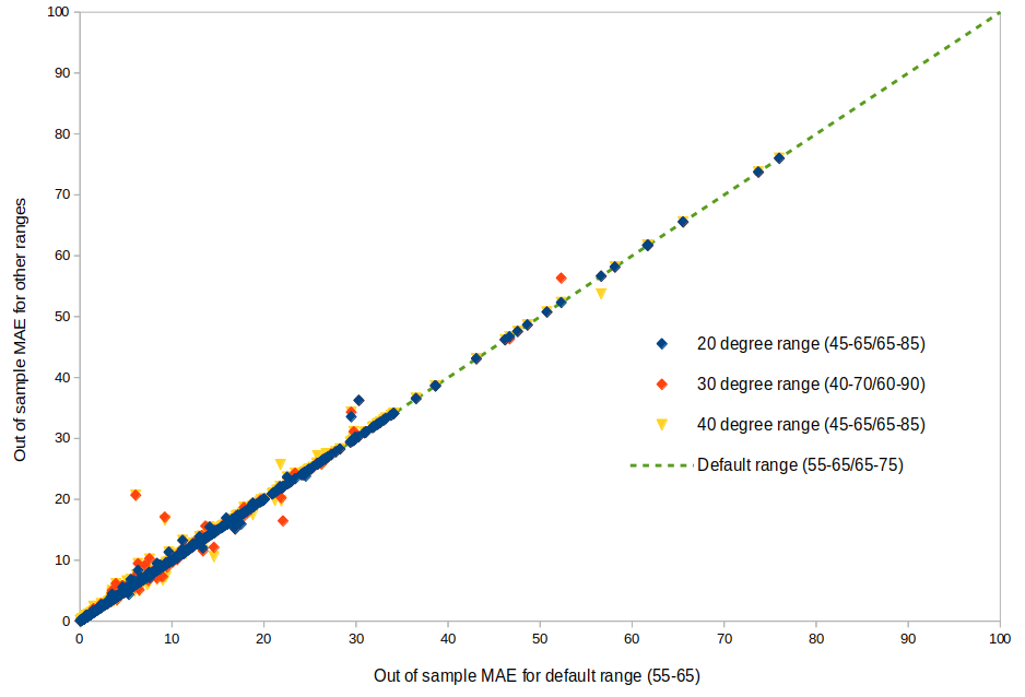
TEST RESULTS

Background
The CalTRACK model uses variable base degree day regression to model baseline and reporting period energy use. Part of this process involves fitting a number of models across a range of heating and cooling balance points. One decision point that is typically decided by an analyst, is the actual search range of balance points. A larger search range requires more computational time and may yield non-physical results (e.g. if the heating balance point is 100 F), especially when data quality is subpar. On the other hand, a search range that is too narrow may lead to poor model fit.

Dataset
Billing data from 1000 residential buildings in Oregon and daily data from 1000 participants in an HVAC program in California.

Tested parameters
Default Caltrack methods were used with different search ranges for the HDD and CDD balance points.

Results

Caltrack models were fit to the Oregon building usage dataset using 4 balance point search ranges:
• 10 degree spread: 55-65 heating, 65-75 cooling
• 20 degree spread: 45-65 heating, 65-85 cooling
• 30 degree spread: 40-70 heating, 60-90 cooling
• 40 degree spread: 40-80 heating, 50-90 cooling

Figure 1 shows the distribution of best-fit HDD balance points for three of those ranges. It is clear that when the search grid is constrained, many models tend to settle at either end of the search range (e.g. for the default search range, almost 30% of buildings have an HDD balance point of exactly 65 F). When the search range is expanded, the distribution of best-fit balance points tends towards a Gaussian distribution (centered at 63 F for this particular dataset). Therefore, we can conclude that a search grid that is too constrained may result in sub-optimal model fits.

Interestingly, Figure 2 demonstrates that even though many models may be sub-optimal, the effect on out-of-sample model performance is marginal. Only a handful of models see a significant change in out-of-sample mean absolute error in predictions and the change in overall performance for the sample is negligible.

Figure 1. Effect of balance point search range on distribution of best-fit HDD balance points.

Figure 2. Effect of balance point search range on out of sample mean absolute errors (MAE)

In a separate study, the effect of the balance point range on estimated savings was also analyzed using a dataset of HVAC program participants. Baseline models were fit to the full set of program participants five times, varying the search range for the HDD balance point and keeping all other parameters constant. Figure 3 shows clearly that the HDD search range has a negligible effect on calculated savings.

Figure 3. Effect of HDD balance point search range on program savings.

We also tested several search increments between 1 and 4 F and in general, the fits do not seem to be much affected when the best-fit balance point is off from the optimal one by up to 2 degrees (Figure 4). This implies that having search increments up to 3 degrees is acceptable as it ensures that the optimal temperature will always be within one degree of a point on the search grid.

Figure 4. Effect of varying heating balance point by 1-2 degrees on model fit.

Recommendations

• Expand balance point search range to 40-80 F for heating and 50-90 F for cooling.
• Allow variable search increments up to 3 F, including multipass grid search and non-uniform search increments.

[steevschmidt]

Great data!
These results make sense to me, except for Figure 3...
Can anyone explain why all five results in this chart look absolutely identical?
I would have expected different types of energy savings (HVAC vs baseline) to produce variations in this test.

[hshaban]

Good question, @steevschmidt . Most models didn't change with an expanded search grid and I think it's just a matter of the dense plot masking the points that did change. I went back and pulled out a 100 buildings where the optimal balance point and total savings did change and as you can see below the changes are very modest. It appears that when we change the balance point search grid, the savings breakdown (heating vs cooling vs baseload) does change quite a bit, however, the aggregate savings are relatively unchanged (usually only a 2-3% change). I'll dig in deeper when I get an opportunity.

[bkoran]

One comment about this: Since we will eventually, if not now, be concerned with the timing of savings, e.g. the load shape of savings, and since you wrote that the savings breakdown (heating vs cooling vs baseload) does change quite a bit, getting the appropriate balance or change point may be much more important than just for total savings, especially for interval data. Bill Koran, P.E., CMVP SBW Consulting, INC<http://www.sbwconsulting.com/> 503-974-9741 From: hshaban [mailto:notifications@github.com] Sent: Thursday, March 1, 2018 11:52 AM To: CalTRACK-2/caltrack Cc: Bill Koran; Comment Subject: Re: [CalTRACK-2/caltrack] Expanded balance point search range (#72) Good question, @steevschmidt<https://github.com/steevschmidt> . Most models didn't change with an expanded search grid and I think it's just a matter of the dense plot masking the points that did change. I went back and pulled out a 100 buildings where the optimal balance point and total savings did change and as you can see below the changes are very modest. It appears that when we change the balance point search grid, the savings breakdown (heating vs cooling vs baseload) does change quite a bit, however, the aggregate savings are relatively unchanged (usually only a 2-3% change). I'll dig in deeper when I get an opportunity. [image]<https://user-images.githubusercontent.com/13769526/36866252-a5dc1be2-1d46-11e8-847e-39576d7a4425.png> — You are receiving this because you commented. Reply to this email directly, view it on GitHub<#72 (comment)>, or mute the thread<https://github.com/notifications/unsubscribe-auth/Ai08ipbKJXlYS7LRLuCoPq3CYNRQHoJOks5taFFCgaJpZM4R1exa>.

[steevschmidt]

Hassan wrote:

... savings breakdown (heating vs cooling vs baseload) does change quite a bit, however, the aggregate savings are relatively unchanged ...

If you have an inaccurate disaggregation of heating & cooling loads, and significant changes in weather between the base and reporting years, I believe your savings calculations will be inaccurate.

[hshaban]

@bkoran @steevschmidt I agree that we'd ideally get an accurate load disaggregation. The results show that for some buildings, the balance points and load disaggregation change when expanding the search range, but we don't have the ground truth. The question raised by this issue is what search range we should explore when selecting models. Does using a wide search range give us a better chance at finding the best balance point or is a constrained one more appropriate? Your thoughts?

[steevschmidt]

Does using a wide search range give us a better chance at finding the best balance point or is a constrained one more appropriate? Your thoughts?

I think wider is better, but for balance points outside of expected ranges more work can (& should?) be done. For example, I mentioned pool heating during today's call. There are homes with two different heating balance points throughout the year: one very high for pool heating during an extended summer swim period, and another during the "home heating only" parts of the year. Depending on whether your goal is "fit" or "accurate load disaggregation", one may chose different approaches.

[margaretsheridan]

I also would like to emphasize the quality of the temperature data going into the model - particularly for hourly estimation. I performed correlations of hourly weather station data by proximity to fill in missing data and to help identify outliers. This cleaning activity greatly improved my adjusted R squared values. I am now using a third-party product to ensure the quality of the weather data. This should be foundational and should be part of a standardized process.

[hshaban]

I think wider is better, but for balance points outside of expected ranges more work can (& should?) be done.

I agree with you @steevschmidt . A wider range makes sense and we could take anomalous balance points into account with building qualification (those buildings may need custom models separate from the default Caltrack path)

[hshaban]

@margaretsheridan Definitely useful input. If you don't mind, could you add some thoughts around weather data cleaning and how to treat missing values in Issue #65? Or any relevant literature/documentation would also help.

[bkoran]

Also agree with margaretsheridan. We've seen cases where nearby NWS sites don't track each other; there are anomalous deviations for a period of time of months or more. (I've also seen where temperatures deviate dependent upon which way the wind is blowing, which is not anomalous.) This is in addition to the dropouts and bad data. Data cleaning, in general, is an important issue.

[bkoran]

Several related comments: These models will almost inevitably be used in ways you don’t expect. For example, I have seen similar models used in industrial applications. In those cases, the constrained search range could be far from the truth. More below about how constrained searches can be an issue. There is little merit, in my view, to using a narrow search range, nor to use a wide tolerance. A search for a single change point is pretty fast: Checking using ECAM, with a search resolution of 0.05 ºF: 365 (daily) data points: less than 0.5 seconds 5110 (hourly) data points: less than 1.0 seconds (I’m not using a decent resolution timer to get a better number.) Of course, finding 2 change points greatly increases the iterations. 846 (hourly) data points: less than 3 seconds with a resolution of 0.18 ºF; add less than 1 second to get the resolution <0.02 ºF. (Yes, I know these resolutions are much, much finer than we actually know the temperatures at the site.) This is in a spreadsheet with interpreted code and worksheet functions! With compiled code and better programmers than me, on a server, maybe you can probably beat that by two orders of magnitude? These searches use the full range of the data, merely requiring at least 3 points on each side of a change point. Also, there is no reason to use degree-days with daily or hourly data. Just use temperature directly. There is no loss of information since degree-days are already at the daily level. Why use an intermediate calculation? It is extra, less transparent, and doesn’t plot as easily. (In most climates, we have seen very little if any value to even using degree-days at the monthly level instead of monthly average temperature, but theoretically degree-days should be better, and likely is in CA climates.) Another point is that you need to use a wide search range because the temperatures found are not necessarily heating and cooling base temperatures: For example, in a residence with a heat pump with supplemental electric heat, there will be 2 heating slopes and hence 2 heating coefficients: One coefficient at moderately cool temperatures for heat pump heating, and a different coefficient at colder temperatures when the supplemental electric heat kicks in. Similar things occur on the cooling side with economizers and mechanical cooling. Yet another change point can occur due to equipment running out of capacity. This can occur at quite cold or quite warm temperatures. A final, less important point: The best fit balance point temperature or change point is not always the maximum likelihood change point. This doesn’t seem to be an issue with higher-frequency data, but it can rarely be an issue with monthly billing data, and can result in one of those change points that doesn’t seem to make sense. I’ve never implemented it, but a maximum likelihood change point might avoid a few change points that fall outside of expectations. Bill Koran, P.E., CMVP Sr. Energy analytics engineer SBW Consulting, Inc. bill.koran@sbwconsulting.com<mailto:bill.koran@sbwconsulting.com> 503-974-9741 3945 parker rd. west linn, or 97068 www.SBWConsulting.com<http://www.sbwconsulting.com/> From: hshaban [mailto:notifications@github.com] Sent: Thursday, March 1, 2018 1:29 PM To: CalTRACK-2/caltrack Cc: Bill Koran; Mention Subject: Re: [CalTRACK-2/caltrack] Expanded balance point search range (#72) @bkoran<https://github.com/bkoran> @steevschmidt<https://github.com/steevschmidt> I agree that we'd ideally get an accurate load disaggregation. The results show that for some buildings, the balance points and load disaggregation change when expanding the search range, but we don't have the ground truth. The question raised by this issue is what search range we should explore when selecting models. Does using a wide search range give us a better chance at finding the best balance point or is a constrained one more appropriate? Your thoughts? — You are receiving this because you were mentioned. Reply to this email directly, view it on GitHub<#72 (comment)>, or mute the thread<https://github.com/notifications/unsubscribe-auth/Ai08isB3GAn7JL83ugJeCnUUuzVvX9NPks5taGgXgaJpZM4R1exa>.

[bkoran]

Again, I don't see a strong rationale for constraining the grid search.

Related to this, it is important that the daily methods are not limited to a single slope for heating and a single slope for cooling. This often doesn't match the physics of the building and can result in poorer fits. It may not mean that savings estimates will change greatly, but it probably will: Least squares slopes tend to aim at the points that are at the extreme cold or extreme warm temperatures. However, the majority of temperatures are in the more moderate range. So the slopes, and hence predictions will be off. Attached is a model for gas; similar situations for electricity can also occur.

You may consider that the attached gas use could be modeled with a negative coefficient for the cooling slope. That is possible, but the point is that a model limited to 2 slopes, or 2 slopes plus a flat range between the balance/change point temperatures, is not always sufficient for daily data.

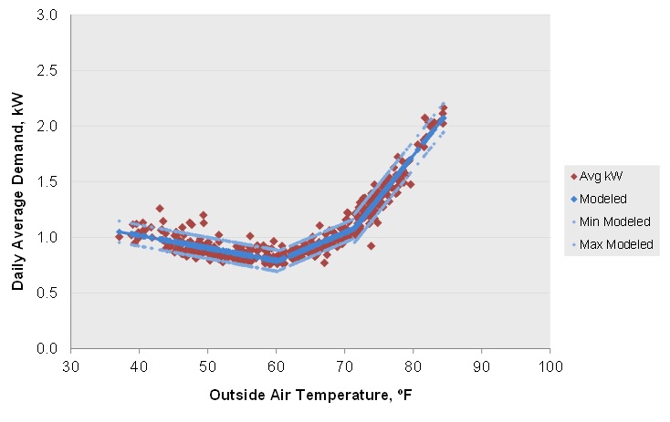
Since I think these methods are planned to also be used for groups of homes, attached is a model of ~200 homes, showing 3 slopes. This is from Figure 16 in

[bkoran]

Since I think these methods are planned to also be used for groups of homes, attached is a daily model of ~200 homes, showing 3 slopes. This is from Figure 16 in
http://www.calmac.org/publications/AMI_Report_Vol_2_Appendices_FINAL.pdf

[mcgeeyoung]

@bkoran I've been thinking a lot about the "elbow" issue. There's no doubt that it's observable. There are three questions that seem important to answer about it. First, what does the poor model fit do to savings estimates? If the model errors are evenly distributed over the course of a year, would we be concerned about its effects? Second, are there quantitative criteria for determining when an "elbow" would be valuable to search for? Should it be default? Should it be configurable? Should it be based on probability of occurrence? Finally, how do we test for this? The image you showed above is a kW function, not a kWh function. Is that relevant?

It strikes me that when we get to hourly modeling that this is going to be a much more relevant conversation. Don't give up on this. We are benefitting from your insights on this issue. We just need a way to generalize it and test it so that it can be fit into the methods specification in a clear, broadly applicable fashion.

[bkoran]

I can't answer most of your questions very well. I covered savings up above; I do think it can have an effect. It could be that it's effects could be minimized by using a different fit than least squares; not sure about that.
There are physical characteristics when an "elbow" should be searched for, but I don't know how to know when analytically except by brute force trying and testing significance.
I don't think it should be default; it is common but not the most common.
Configurable? Don't know what you mean.
kW vs. kWh is just time integration; don't think it matters

[bkoran]

A bit more--this is more specific to hourly models, although it can affect daily models:
One of the most common measures in building commissioning is improving economizer operation, i.e. cooling with outside air. Economizers operate at moderate temperatures, from the cooling change/balance point up to somewhere between 62 and 73 degF, depending on climate and humidity. In a model they are characterized as having a steeper slope than the rest of the cooling. Since the savings are at temperatures close to the change/balance point, I believe the effect of this improvement would be all but invisible if only a single slope is used for cooling. Maybe that is good enough in a whole building project with many measures, but this is a very common measure, and the 2 slopes are often obvious when an economizer is performing well. (Corollary is that the base case often doesn't show it, but the post case does.)

The first 2 charts below are EnergyPlus models of a DOE prototype building. The first is a daily model, the second hourly. The third chart is an hourly model of a real building.

[margaretsheridan]

When I was forecasting hourly system load for systems operations at SMUD years ago, I used multiple techniques including a regression with a third order polynomial for the temperature-load relationship. This would track fairly well with piecewise linear load-temp relationship. The greater simplicity of modeling would need to be examined relative to any loss in accuracy.

[hshaban]

This update has been integrated in CalTRACK 2. Closing this issue