TutorialSmallHeliostatsTower
This tutorial explains:
- How to use “Tracker_Heliostat” plug-ins to embed solar tracking behavior within the Tonatiuh model of a solar concentrating system.
- How to use the scripting capabilities of Tonatiuh to automate the use of the program to simulate the optical behavior of a tracking solar concentrating system as a function of the sun position in the sky.
- How to use Mathematica to post-process the results generated by Tonatiuh to compute the solar flux distribution incident upon a flat rectangular surface.
- How to combine Tonatiuh and Mathematica capabilities to generate a optical efficiency matrix to characterize the optical behavior of a tower system.
For a given position of the sun in the sky and a given value of the direct solar irradiance, what we want to estimate is the heliostat field solar collection efficiency. This efficiency is defined as the ratio between the amount of solar energy that reaches the central receiver input aperture plane and the maximum amount of solar energy that could reach the mirrored surfaces of the heliostat field.
From the above definition of the heliostat field solar collection efficiency, it follows that this efficiency is a function of the heliostat reflectivity, the atmospheric transmissivity, the distances from the heliostats to their corresponding aiming points in the central receiver input aperture plane, the angle of incidence of the direct solar radiation upon the heliostats' mirrors (cosine factor) and the blocking and shadowing among heliostats.
To simplify matters, for the purpose of this tutorial, we will assume that all heliostats in the the heliostat field have the same reflectivity. If this is the case, the average heliostat reflectivity will appear in both the numerator and the denominator of the expression to estimate the solar collection efficiency of the heliostat field, and, thus, it will disappear from the expression. This implies that, in this specific case and for the specific assumptions we are considering, any average reflectivity value greater than zero will suffice for the purpose of calculating the heliostat field collection efficiency. Thus, we set the average heliostat reflectivity to one.
Furthermore, for simplicity, we assume that the atmospheric losses from the heliostats to the central receiver aperture plane, due to atmospheric transmittance, are just one and the same small constant fraction for all heliostats, whatever their position in the field. With this assumption, as in the average heliostat reflectivity case, the atmospheric transmittance will reduce to an average value that will show up both in the numerator and denominator of the heliostat field solar collection efficiency calculation, canceling each other out. Because of this, for this tutorial, we set the atmospheric transmittance to one.
With this simplifying assumptions the heliostat field solar collector efficiency will only depends, at any given instance of the day, on the cosine factor and the shadowing and blocking.
What we want to illustrate with this Tutorial is how you can use Tonatiuh to generate a look-up table or matrix of heliostat field solar collection efficiency values as a function of the two angles that define the Sun position in the sky (solar azimuth and zenith angle).
This look-up table will allow you to interpolate, for any given sun position, the solar collection efficiency of the tower system under analysis. An information that is relevant for many purposes, such as, for instance, to establish a quantitative metric to drive a heliostat field layout automatic optimization process.
The tower system that we want to model in this tutorial consist of:
- A dense heliostat field of 500 small 5 m x 5 m one-facet heliostats,
- A tower, and
- The input aperture of the solar central receiver.
Figure 1 shows the basic layout the heliostat field and the relative location of the tower. As it can be seen, the heliostats form an array of 25 columns and 20 rows, regularly spaced.
From the dimensions presented in the figure, knowing that the distance between the centers of the facets of two adjacent heliostats located in a row, or column, is 5.5 meters, it is straightforward to compute the relative coordinates of the center of the facet of each heliostat in the field. Obviously, to do that you need to select the position of the origin of coordinates. For convenience, we fix this origin at the center of the heliostat field, with the positive x-axis towards the East, the postive y-axis towards the zeinth, and the positive z-axist towards the North.
 |
|---|
| Figure 1. Tower system layout. |
We will assume that all of the heliostats will aim to the center of the input aperture, which is a 10 meters by 10 meters target with its center 130 m above the plane defined by the centers of the facets of the heliostats.
To model the input aperture of the central receiver do the following:
- In Tonatiuh's Tree View click on the TSeparatorKit "RootNode".
- Go to the plug-ins Menu Bar and click on the TSeparatorKit icon, to add a new TSeparator as a new children of "RootNode".
- Double click on the newly created TSeparatorKit node and change its name to "Target_Frame".
- With the "Target_Frame" node selected, go to the "Transform" properties dialog, just below the tree view, and set the transform properties as follows:
translation        0 130 74.25
rotation           -1 0 0 1.5707964
scaleFactor        1 1 1
scaleOrientation   0 0 1 0
center             0 0 0
- With the TSeparatorKit "Target_Frame" selected in the Tree View, go to the plug-ins Menu Bar and click on the TShapeKit icon to create a TShapeKit node under the "Target_Frame" node.
- By default this newly created TShapeKit will be labeled "TShapeKit1", double click on the name and change it to "Target_ShapeKit".
- With the "Target_ShapeKit" node selected, go to the plug-ins Menu Bar and click on the "!Flat_rectangle" TShapeNode icon to add a TShapeNode to the "Target_ShapeKit".
- By default this newly created TShapeNode will be labeled "Flat_Rectangle", keep the name.
- Click on the "Flat_Rectangle" TShapeNode to select it. Go to the “ShapeFlatRectangle” dialog that will appear below the Tree View and set the values of the parameters that define this shape node to:
width      10
height     10
activeSide FRONT
- Under the "Target_Frame" TSeparatorKit click the TShapeKit node labeled "Target_ShapeKit" to select it.
- With the "Target_ShapeKit" selected, go to the Tonatiuh plug-ins Menu Bar and select the Specular_Standard_Material icon.
- After the new material node is created within the "Target_ShapeKit" node, click on it to select it.
- With the "Specular_Standard_Material" node selected go to the MaterialStandardSpecular properties dialog that will appear below the Tree View, and set the values of the parameters that define this material node to:
m_reflectivity   0
m_sigmaSlope     2
m_distribution   PILLBOX
m_ambientColor   0 0 0
m_diffuseColor   0 0 0
m_specularColor  0 0 0
m_emissiveColor  0 0 0
m_shininess      0
m_transparencey  0
To model the tower do the following:
- In Tonatiuh's Tree View click on the TSeparatorKit "RootNode".
- Go to the plug-ins Menu Bar and click on the TSeparatorKit icon, to add a new TSeparator as a new children of "RootNode".
- Double click on the newly created TSeparatorKit node and change its name to "Tower_Frame".
- With the "Tower_Frame" node selected, go to the "Transform" properties dialog, just below the tree view, and set the transform properties as follows:
translation        0 0 76.35
rotation           0 0 1 0
scaleFactor        1 1 1
scaleOrientation   0 0 1 0
center             0 0 0
- With the TSeparatorKit "Tower_Frame" selected in the Tree View, go to the plug-ins Menu Bar and click on the TShapeKit icon to create a TShapeKit node under the "Tower_Frame" node.
- By default this newly created TShapeKit will be labeled "TShapeKit1", double click on the name and change it to "Tower_ShapeKit".
- With the "Tower_ShapeKit" node selected, go to the plug-ins Menu Bar and click on the "Cone" TShapeNode icon to add a cone TShapeNode to the "Tower_ShapeKit".
- By default this newly created TShapeNode will be labeled "Cone", keep the name.
- Click on the "Cone" TShapeNode to select it. Go to the “ShapeCone” dialog that will appear below the Tree View and change the values of of the parameters that define this shape node to:
baseRadius  3
topRadius   2
height      130
phiMax      6.2831855
activeSide  OUTSIDE
 |
|---|
| Figure 2. Tonatiuh's GUI after modeling the target and the tower. |
Figure 2 shows the GUI of Tonatiuh after finishing the above steps. In four different 3D views you can see, from different point of views, the 10 m x 10 m flat rectangle modeling the aperture and the 130 meters tall cone modeling the tower. Furthermore, in the Tree View, you can see the tree-node structure that makes up the current definition of the solar concentrating system, which up this point is only composed of the central receiver input aperture model or target and the tower model.
As mentioned before, the heliostat field we want to model is composed of 500 small 5 m x 5 m one-facet heliostats, distributed in a rectangular array of 20 rows and 25 columns.
Please, to model the heliostat field layout do the following:
- In Tonatiuh's Tree View, click on the "RootNode" separator node to select it.
- With the "RootNode" selected go to the Menu Bar and click on the TSeparatorKit icon, this will have the effect of inserting a new TSeparatorKit under the node "RootNode".
- Change the name of the newly created TSepartorKit from "TSeparatorKit1" to "HeliostatField_Frame".
- Repeat the following two steps 20 times, replacing "XX" in the name "RowXX_Frame" by the number of the repetition: * Select the node "HeliostatField_Frame" and go to the Menu Bar to insert another TSeparatorKit node below it. * Change the name of the newly created TSeparatorKit node to "RowXX_Frame".
- After the 20 TSeparatorKit nodes "RowXX_Frame" are created change their "Transform" so that the values of their "translation" parameters are as follows:
Row01_Frame: translation   0 0 -52.3
Row02_Frame: translation   0 0 -46.8
Row03_Frame: translation   0 0 -41.3
Row04_Frame: translation   0 0 -35.8
Row05_Frame: translation   0 0 -30.3
Row06_Frame: translation   0 0 -24.8
Row07_Frame: translation   0 0 -19.3
Row08_Frame: translation   0 0 -13.8
Row09_Frame: translation   0 0 -8.3
Row10_Frame: translation   0 0 -2.8
Row11_Frame: translation   0 0 2.8
Row12_Frame: translation   0 0 8.3
Row13_Frame: translation   0 0 13.8
Row14_Frame: translation   0 0 19.3
Row15_Frame: translation   0 0 24.8
Row16_Frame: translation   0 0 30.3
Row17_Frame: translation   0 0 35.8
Row18_Frame: translation   0 0 41.3
Row19_Frame: translation   0 0 46.8
Row20_Frame: translation   0 0 52.33
- Once the translation parameters of the transforms of the 20 TSeparatorKit nodes are updated, click on the TSeparatorKit "Row01_Frame" to select it.
- With the "Row01_Frame" selected in Tonatiuh's Tree View, go to the Menu Bar and click on the TSeparatorKit icon, to insert a new node of that kind under the "Row01_Frame".
- Rename the TSeparatorKit just created to "Row".
- Select the TSeparatorKit "Row" and create under it 25 TSeparatorKit nodes, named "HeliostatXX_Frame", where "XX" goes from 1 to 25.
- After the 25 TSeparatorKit nodes "HeliostatXX_Frame" are created change their "Transform" so that the values of their "translation" parameters are as follows:
Heliostat01_Frame: translation   -66 0 0
Heliostat02_Frame: translation   -60.5 0 0
Heliostat03_Frame: translation   -55 0 0
Heliostat04_Frame: translation   -49.5 0 0
Heliostat05_Frame: translation   -44 0 0
Heliostat06_Frame: translation   -38.5 0 0
Heliostat07_Frame: translation   -33 0 0
Heliostat08_Frame: translation   -27.5 0 0
Heliostat09_Frame: translation   -22 0 0
Heliostat10_Frame: translation   -16.5 0 0
Heliostat11_Frame: translation   -11 0 0
Heliostat12_Frame: translation   -5.5 0 0
Heliostat13_Frame: translation   0 0 0
Heliostat14_Frame: translation   5.5 0 0
Heliostat15_Frame: translation   11 0 0
Heliostat16_Frame: translation   16.5 0 0
Heliostat17_Frame: translation   22 0 0
Heliostat18_Frame: translation   27.5 0 0
Heliostat19_Frame: translation   33 0 0
Heliostat20_Frame: translation   38.5 0 0
Heliostat21_Frame: translation   44 0 0
Heliostat22_Frame: translation   49.5 0 0
Heliostat23_Frame: translation   55 0 0
Heliostat24_Frame: translation   60.5 0 0
Heliostat25_Frame: translation   66 0 0
- Once the translation parameters of the transforms of the 25 TSeparatorKit nodes are updated, click on the TSeparatorKit "Heliostat01_Frame" to select it.
- With the "Heliostat01_Frame" selected in Tonatiuh's Tree View, go to the Menu Bar and click on the TSeparatorKit icon, to insert a new node of that kind under the "Heliostat01_Frame".
- Rename the TSeparatorKit just created to "Heliostat", and with it selected go to the Menu Bar and click on the "Heliostat_tracker" icon to insert a node of that type under the "Heliostat" TSeparatorKit node.
- After creating the Heliostat_tracker node under the "Heliostat" TSeparatorKit node, select the Heliostat_tracker node and in the "TrackerHeliostat" dialog that appears just below the Tree View set the value of the parameter "aimingPoint" as follows:
aimingPoint 0 130 74.25
- Now, right-click on the "Heliostat" TSeparatorKit node and in the pop-up menu that will be shown as a result select "copy" to copy the "Heliostat" node and its children, which in this case is only the Heliostat_tracker node. Alternatively, click on the "Heliostat" node and with the node selected in the Tree View push "Ctrl + c".
- After you have copied the "Heliostat" node and its child (the Heliostat_tracker node) to the clip-board, select one by one the remaining 24 "HeliostatXX_Frame" nodes, which are children of the node "Row", and in each one of them do "Ctrl + v" to paste a copy of the "Heliostat" node below each those TSeparatorKit nodes.
- After executing the previous step, every "HeliostatXX_Frame" TSeparatorKit node, which is below the "Row" TSeparatorKit node, should have a "Heliostat" node as a child. Once this is achieved, select the "Row" TSeparatorKit and do "Ctrl + c" to copy it to the clip-board.
- With the "Row" TSeparatorKit and its 25 "HeliostatXX_Frame" as its children copied to the clip-board, select each one of the 19 remaining "RowXX_Frame" nodes and do "Ctrl + v" to paste a copy of "Row" below each one of them.
After executing the steps above, the origins of the local coordinate frames of each one of the heliostats in the field will be specified. Furthermore all of those frames will have a "heliostat tracker" node that will change their orientation so that a central ray coming from the sun and incident upon their origins will be reflected towards the defined aiming point, which in this case is the center of the central receiver aperture (0 130 74.25).
However, those local heliostat frames modeled in Tonatiuh as TSeparatorKits, do not include yet the physical model of the heliostat, which in this tutorial is composed of a TShapeKit node, a TShape node, and a TMaterials node. That is the reason why at this stage in the modeling of the heliostat field, no heliostat is shown in Tonatiuh's 3D view.
The heliostat to model is an small one-facet heliostat. Only the mirror needs to be modeled in Tonatiuh, since for a given heliostat the supporting mirror structure and tracking mechanism is not expected to cast relevant shadows on nearby heliostats.
The heliostat mirror is assumed to be a 5 meters by 5 meters spherical rectangular mirror. Since, for the heliostat field the characteristic slant range of a heliostat is 150 m, the radius of the spherical mirror will be 300 m. Therefore, to model the heliostat in Tonatiuh, please, do the following:
- Go to the Tree View of Tonatiuh and expand the "HeliostatField_Frame" TSeparatorKit node. Then, expand the "Row01_Frame" TSeparatorKit node. Then, expand the "Row" TSeparatorKit node. Then, expand the "Heliostat01_Frame" TSeparatorKit node, and click on the "Heliostat" TSeparatorKit node to select it.
- Once the "Heliostat" node with the node path "HeliostatField_Frame\Row01_Frame\Row\Heliostat01_Frame" is selected, go to the plug-in Menu Bar and click on the ShapeKit icon to insert a new TShapeKit object below the “Heliostat” TSeparatorKit.
- Expand the “Heliostat” node, if it is not already expanded, to make the newly created TSeparatorKit visible in the Tree View. Once it is visible, double click on to change its name from “TShapeKit1” to “Heliostat_ShapeKit”.
- With the newly created “Heliostat_ShapeKit” TShapeKit selected, go to the plug-in Menu Bar and click on the “!Spherical_rectangle” icon to insert a new “Spherical_rectangle” shape node under the “Heliostat_ShapeKit” node. This new shape node will be created with the default name “Spherical_rectangle”, change it to "Facet_Geometry".
- With the “Facet_Geometry” shape node selected in the Tree View, go to the “ShapeSphericalRectangle” dialog that will appear below the Tree View and set the values of the parameters that define this shape node to:
radius     300
width X    5
widthZ     5
activeSide INSIDE
- Select the "Heliostat_ShapeKit" TShapeKit node and go to the Tonatiuh plug-ins Menu Bar and select the Specular_Standard_Material icon to insert a standard specular material node as a child of the "Heliostat_ShapeKit" node.
- After the new material note is created within the heliostat's TShapeKit, select the material node to change the default material's properties.
- In the MaterialStandardSpecular preperties dialog that will appear below the Tree View, for the purpose of this tutorial, please, change the value of the parameter “m_reflectivity” from 0 to 1.
- Once the first "Heliostat_ShapeKit" node is completed with its two childre nodes: "Facet_Geometry" and "Specular_Standard_Material", this same node has to be "paste-linked" into the 499 remaining "Heliostat" nodes, which are located under the following paths "HeliostatField_Frame!RowXX_Frame\Row!HeliostatYY_Frame", where XX is the row number, which goes from 0 to 20, and YY is the heliostat number in a given row, which goes from 0 to 25.
- To "paste link" the "Heliostat_ShapeKit" node, first copy it to the clip-board, by selecting it and doing "Ctrl + c", then right-click on the "Heliostat" node in which you want to do the "paste link" and, with the "Heliostat" node selected, in the menu that will pop-up select the "Paste Link" option, which is located just below the "Paste" option. By doing "Paste Link" instead of "Paste" you are obtaining a substantial amount of memory savings, since instead of copying 500 times the objects that compose the "Heliostat_ShapeKit" you are adding just 500 references (i.e., pointers) to original objects you created.
 |
|---|
| Figure 3. Modeling the heliostat field in Tonatiuh. |
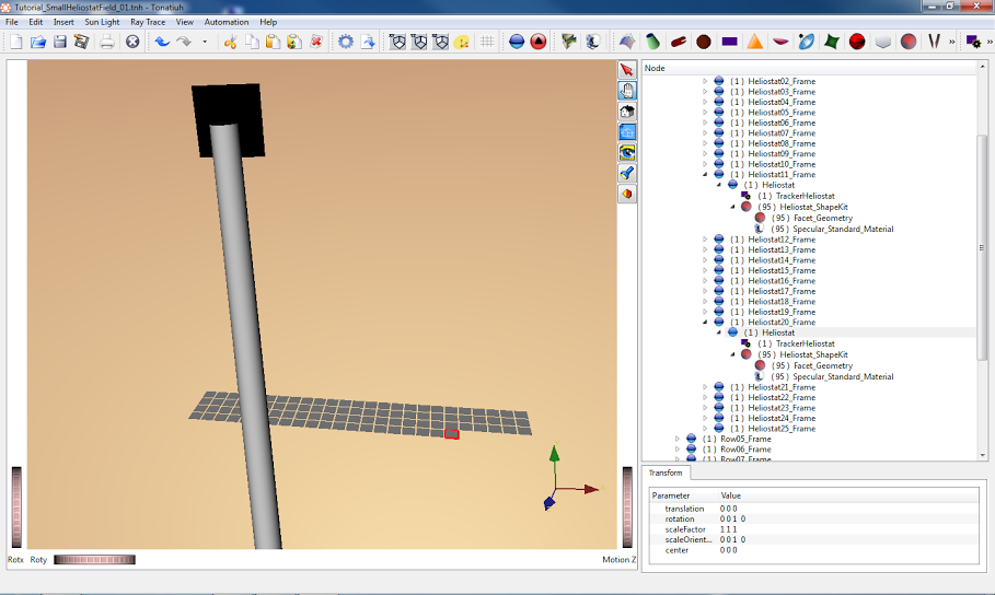
Figure 3 shows Tonatiuh's GUI during the process of "Paste Link" the "Heliostat_ShapeKit" in each one of the 500 nodes named "Heliostat" that are defined in the different rows of heliostats that form the heliostat field. The figure shows the instant in which the "Heliostat_ShapeKit" node has been "paste linked" in the all the nodes named "Heliostat" of the first three rows (further away from the tower) and in 20 "Heliostat" nodes of fourth row. This is the reason the number in parenthesis before the "Heliostat_ShapeKit" name indicates 95, since that number indicates the number of time a given object is referenced within Tonatiuh's physical description model.
 |
|---|
| Figure 4. The heliostat field of 500 one-facet heliostats. |
Figure 4. Shows the Tonatiuh's GUI after the process of "Past Link" the "Heliostat_ShapeKit" in each one of the 500 nodes named "Heliostat" has finished. You can see the 20 rows of 25 heliostats each that define the heliostat field. In the figure, all heliostats are aiming upwards, since the position of the sun and the rest of the characteristics that define the direct solar radiation reaching the heliostats has still to be defined.
To define the characteristics of the direct solar radiation incident upon the solar concentrating system, please, do the following:
- Go to the Main Menu and click on "Sun Light".
- Then, on the water-fall menu that will be presented, click on the "Define SunLight..." option, which should be the only option available for selection.
- Clicking on the "Define SunLight" option will result in the presentation of the pop-up menu named "Define Sun Light" to the user. On the "Sun Shape" tab of the dialog set the tab's parameter values as follows:
Sunshape Type:      Pillbox_Sunshape
irradiance (W/m2):  920
thetaMax (rad):     0.00465
Shape Type:         Flat_Rectangle
width (m):          170
height (m):         150
activeSide:         FRONT
- On the "Sun Position" tab of the dialog set the tab's parameter values as follows:
Azimuth (Degrees North towards East):        0.0
Elevation (Degrees from horizontal plane):  90.0
Distance (m)                             : 200.0
- After all the appropriate "Sun Shape" dialog's values have been defined, click on the pop-up dialog's "OK" button to close the dialog and create the corresponding Light object within Tonatiuh.
After following the steps indicated above, a special node labeled "Light" will appear in Tonatiuh's Tree View. Furthermore, each one of the 500 heliostats that compose the heliostat field will be appropiately oriented so that the direct solar radiation incident upon them will be reflected towards the center of the central receiver aperture.
 |
|---|
| Figure 5. Testing the heliostat trackers in Tonatiuh. |
To verify that all heliostats are properly oriented by their "trackers" just hit the "Execute" button in the Menu Bar to cast a few sun rays over the heliostat field and represent them and their reflections on the heliostats in Tonatiuh's 3D View. Figure 5 shows the results of such a test. As you can see in the figure, the heliostats are appropriately reflecting the direct solar radiation towards the center of the central receiver aperture. With this verification ends the modeling of the small central receiver system considered for this tutorial.
Once the tower system is modeled, Tonatiuh can be used to simulate the system's optical behaviour. With Tonatiuh you can simulate how the system will work under different solar conditions. These conditions are characterized by the Sun position in the sky, which define the main direction of the incoming direct solar radiation, and the direct solar irradiance, which defines the amount of radiant power per unit area normal to the main direction of the incoming solar radiation associated with that radiation.
This work is licensed under a Creative Commons Attribution-Noncommercial-Share Alike 3.0 Unported License
