(Part of Self Driving Car Specialization)
Analysis of 2d bicycle kinematic model and implementation of rear wheel using matlab
As research on autonomous vehicle matures, the subject of consistency across its many levels becomes increasingly important in ensuring the vehicle's safety. Even if each layer is adequately developed separately, an ill-planned vehicle architecture might be exceedingly dangerous. To understand the vehicle models, we will focus on the derivation, analysis, and implementation of a car by simplifying it into a 2D Bicycle Model.
In this repo, we will derive bicycle kinematic model, which is a well-versed model for its performance in describing vehicle motion in normal driving environment. Due to its simplicity and conformance to the nonholonomic restrictions, the model has long been utilised as a viable control-oriented model for cars. The model is called Front Wheel Steering Model, due to changing of front wheel orientation relative to vehicle's heading as shown in Fig 1.
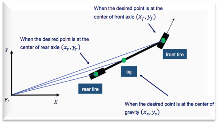
**Fig 1 : 2D Bicycle Kinematics for Front Wheel Steering Model**
To analyze the kinematics of bicycle model, we must select a reference point X, Y which can be placed at the center of the rear & front wheel and at center of gravity (cg).

**Fig2: Bicycle Model**

**Fig3: Model Analysis of Rear Wheel**
Our target is to compute state [x, y, 𝜃, 𝛿], 𝜃 is heading angle, 𝛿 is steering angle. Our inputs are [𝑣, 𝜑], 𝑣 is velocity, 𝜑 is steering rate.
If the desired point is at the center of the rear wheel. First, apply the Instantaneous Center of Rotation (ICR) and then compute state change rate:
ẋ = v * cos (𝜃) ẏ = v * sin (𝜃)
𝜃_dot is equal to rotation rate 𝜔,
𝜔 = 𝑣 / R : R is radius from ICR.
From Figure3, L is the bicycle length and 𝛿 is steering angle, R and 𝜃_dot can be computed as:
R = L / tan(𝛿) 𝜃_dot = 𝑣 / (L / tan(𝛿)) = 𝑣 * tan(𝛿) / L
𝛿_dot is equal to the input 𝜑 (rate of change of steering angle) : 𝛿_dot = 𝜑

**Fig4. Model analysis at Front Wheel**

**Fig5. Model analysis at CG**
As figure 4 shows, the desired point is in the center of front wheel. R can be computed as L / sin(𝛿). We can get the result of changing rate of x, y position.
ẋ = v * cos (𝛿 + 𝜃) ẏ = v * sin (𝛿 + 𝜃)
𝜃_dot = v / R = v / (L/sin(𝛿)) = v * sin(𝛿)/L 𝛿_dot = 𝜑
If the desired point is at the center of gravity or cg. ẋ = v * cos(𝛽 + 𝜃) ẏ = v* sin(𝛽 + 𝜃) For R and 𝜃_dot, S is computed as shown in figure 5: S = L / tan(𝛿) R = S / cos (𝛽) = L / (tan (𝛿) *cos (𝛽) ) 𝜃_dot = v / R = v *tan (𝛿) *cos (𝛽) / L
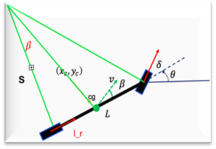
**Fig 6: Analysis for 𝛽**
Furthermore, if we know the distance between the rear wheel and cg denoted as l_r, we can also compute the slip angle 𝛽. Tan (𝛽) = lr / S = lr / ( L / tan (𝛿) ) = lr * tan(𝛿) / L So slip angle: 𝛽 = arctan(lr * tan (𝛿) / L ) 𝛿_dot = 𝜑
Our analyzed bicycle model has the States (outputs) as [x, y, 𝜃, 𝛿], inputs [𝑣, 𝜑], where 𝑣 is the velocity and 𝜑 is steering rate. We can compute the changing rate of [x, y, 𝜃, 𝛿], which is ẋ ẏ, 𝜃_dot, 𝛿_dot.
The derived equation for 2D bicycle model was simulated in using MATLAB Script, by implementing the Rear Wheel equations. To get the final state [x, y, 𝜃, 𝛿], we can use discrete time model:
xt+1 = xt + ẋ * ∆𝑡 yt+1 = yt + ẏ * ∆𝑡
𝜃t+1 = 𝜃t + 𝜃_dot * ∆𝑡 𝛿t+1 = 𝛿t + 𝛿_dot * ∆𝑡
The model start its simulation from initial conditions of , move Left by π/3=60o and then turns Right by π/3=60o.

**Fig 7-8 : Starts from [0 0 π/4] and Turns Left by π/3**

**Fig 9-10 : Model Turns Right by π/3**
A car can be simplified as a 2D bicycle model in a nonholonomic environment for better visualization of vehicle dynamics and control. We developed a bicycle kinematic model for three separate reference locations on the vehicle and implemented it in MATLAB, which allowed us to simulate the model's behavior. This model can be used to create kinematic steering controllers. The bicycle kinematic model provides the foundation for understanding and building self-driving automobile controllers, as well as for developing dynamic vehicle models for any moving system. The Bicycle Model is a classic model that produces a well-versed job in capturing motion of any vehicle in normal driving conditions.


