Planar impact in Eulerian mode
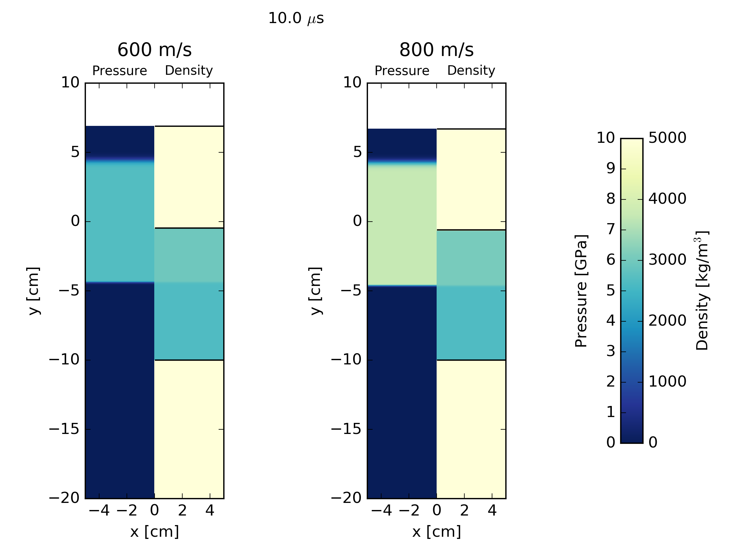
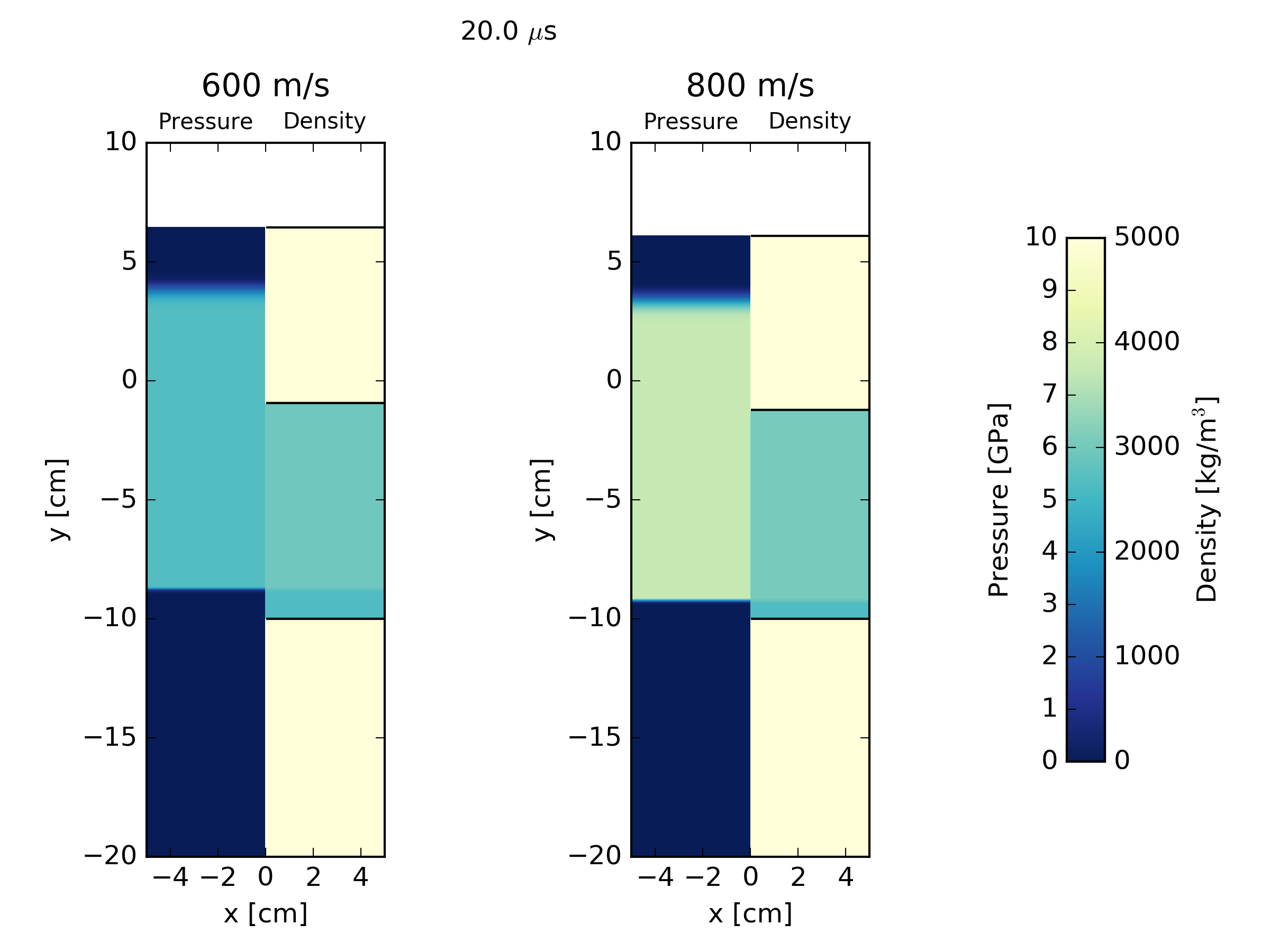
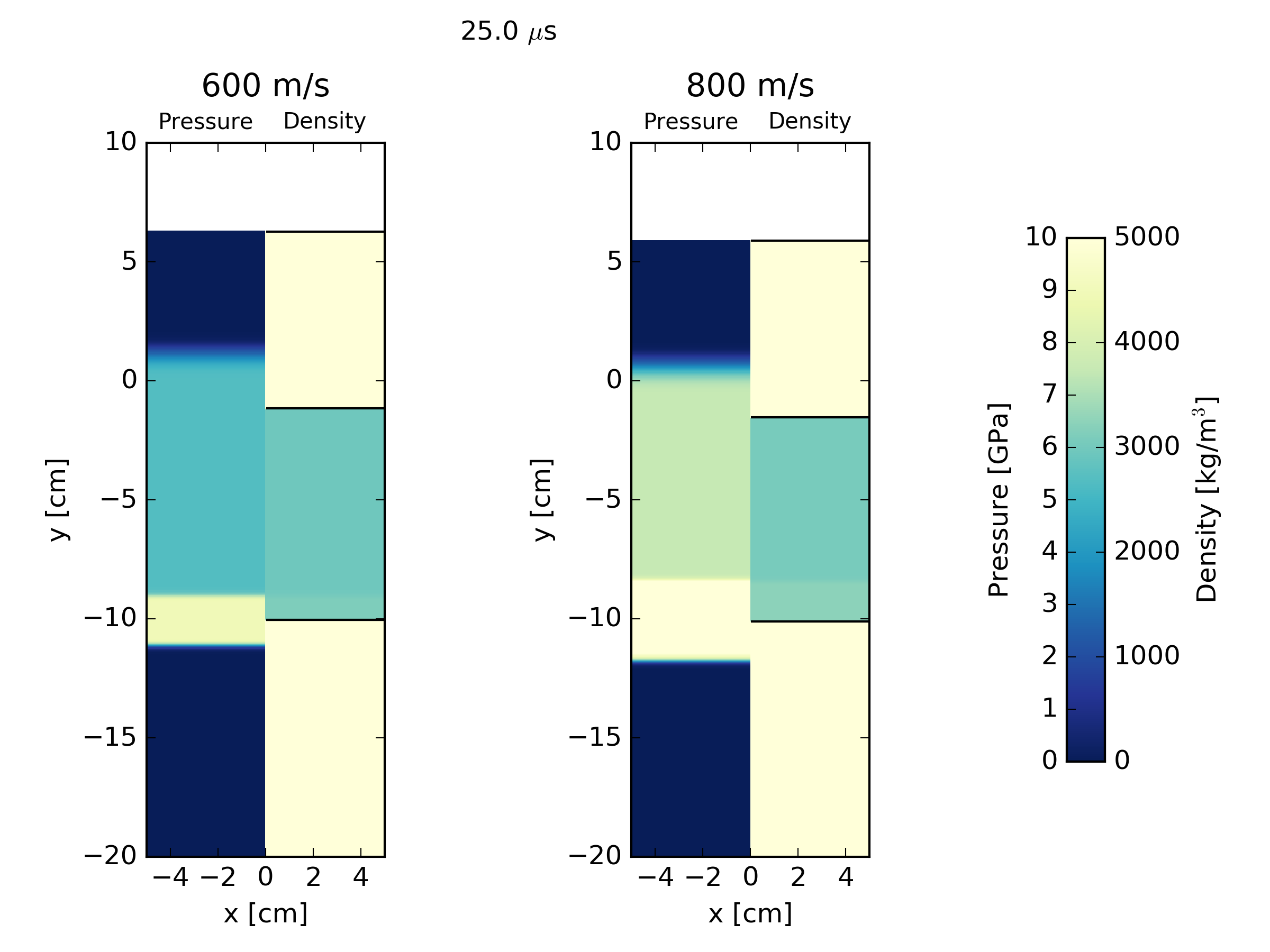
This example simulates, in an Eulerian representation, the impact of an iron plate hitting a quartzite target at 600 m/s, with an iron buffer plate behind the target. The impact initiates a shock wave which travels through the quartzite target. At the interface between the back of the target and an iron buffer plate, the shock wave reflects back into the target and transmits a shock wave into the buffer. As the initial shock wave reaches the back of the impacting plate, a release wave is sent back through the impactor, and into the target.
This example can be used as a template for simple numerical planar-impact experiments analogous to laboratory plate impact experiments. However, note that in this example the strength of each material is neglected.
Go to the relevant example directory
cd /share/examples/planar_eulerian_2D
Run iSALE2D. The simulation will take several minutes, so this should be run in the background.
./iSALE2D &
The exact same simulation, except with a higher impact velocity of 800 m/s, can be run using the command line options:
./iSALE2D -f Planar-800mps --OBJVEL -8.D2 &
The first flag changes the model name (for outputting); the second sets the new object velocity.
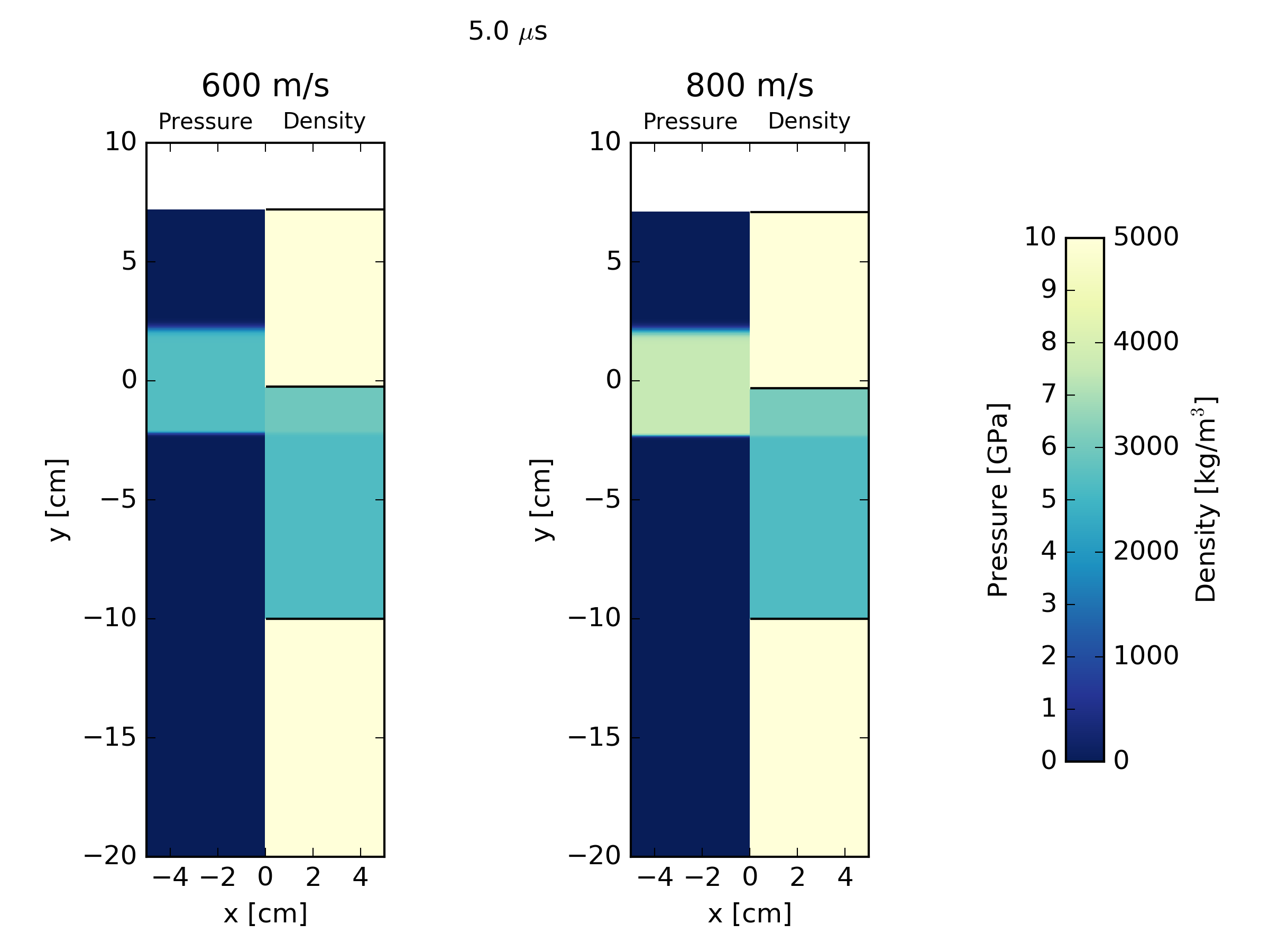
To visualise the density and pressure of the two simulations using pySALEPlot:
python Plotting/DenPre.py
View the images in the DenPre directory.
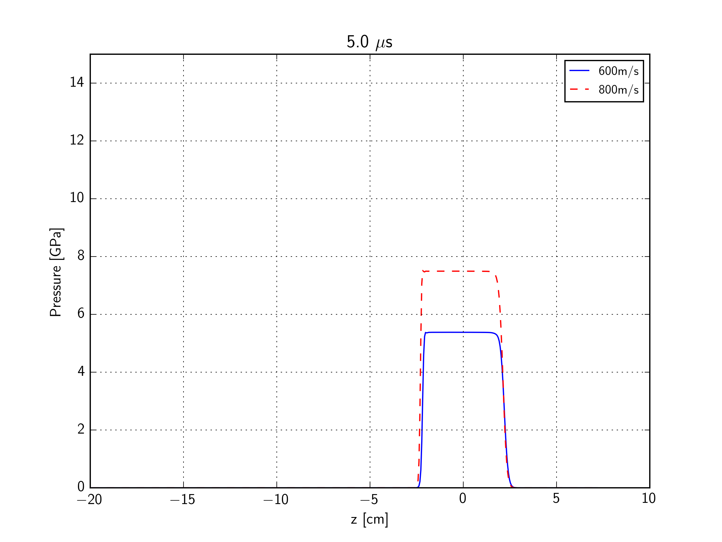
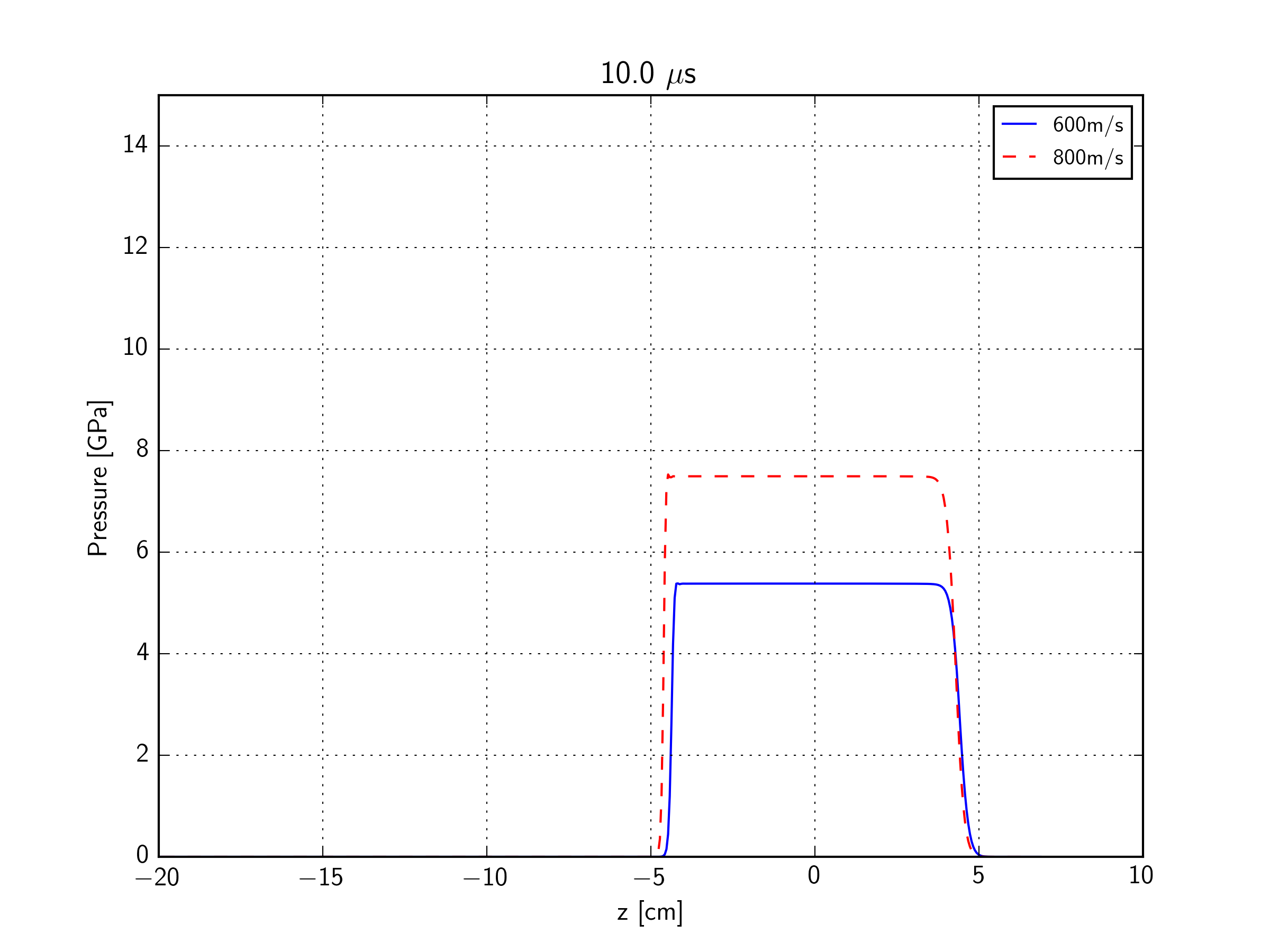
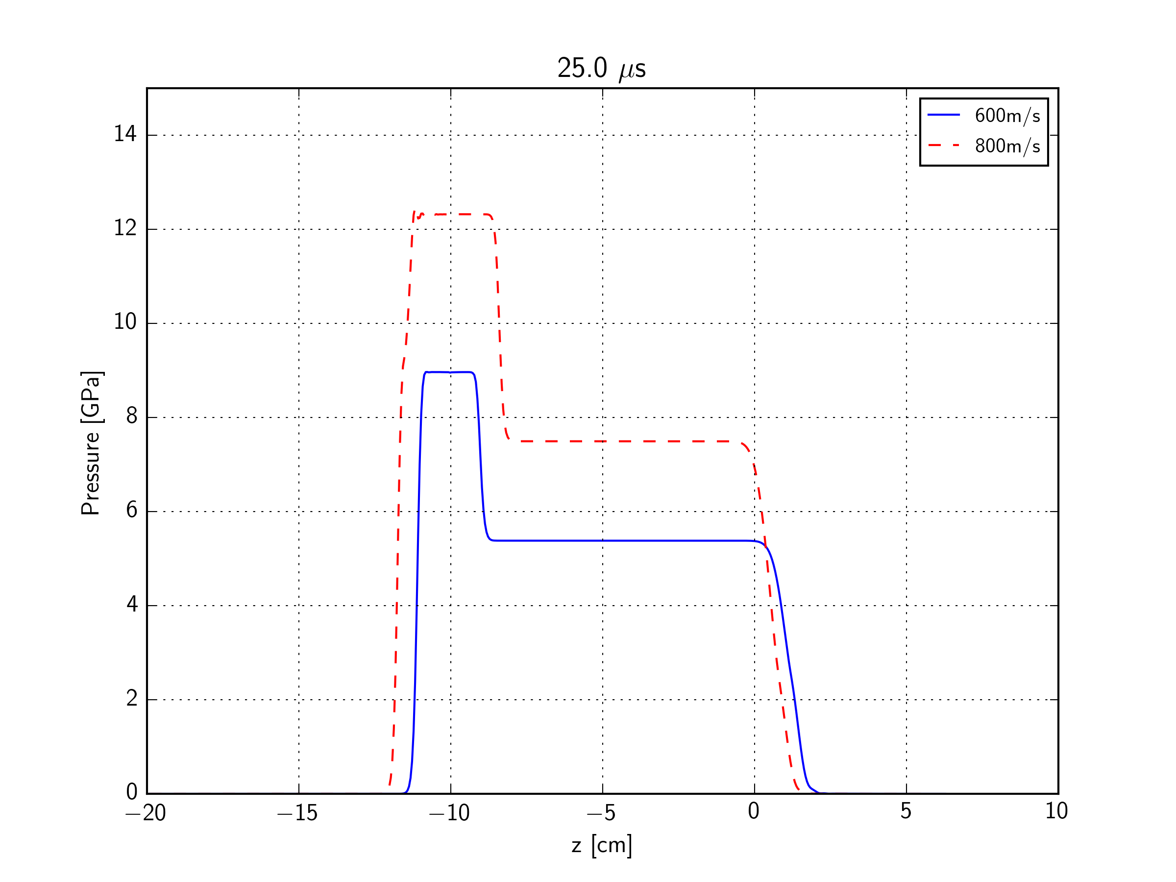
Use pySALEPlot to produce profiles of the pressure pulse as it propagates through the mesh.
python Plotting/PressureProfile.py
And view these images in the PressureProfile directory.
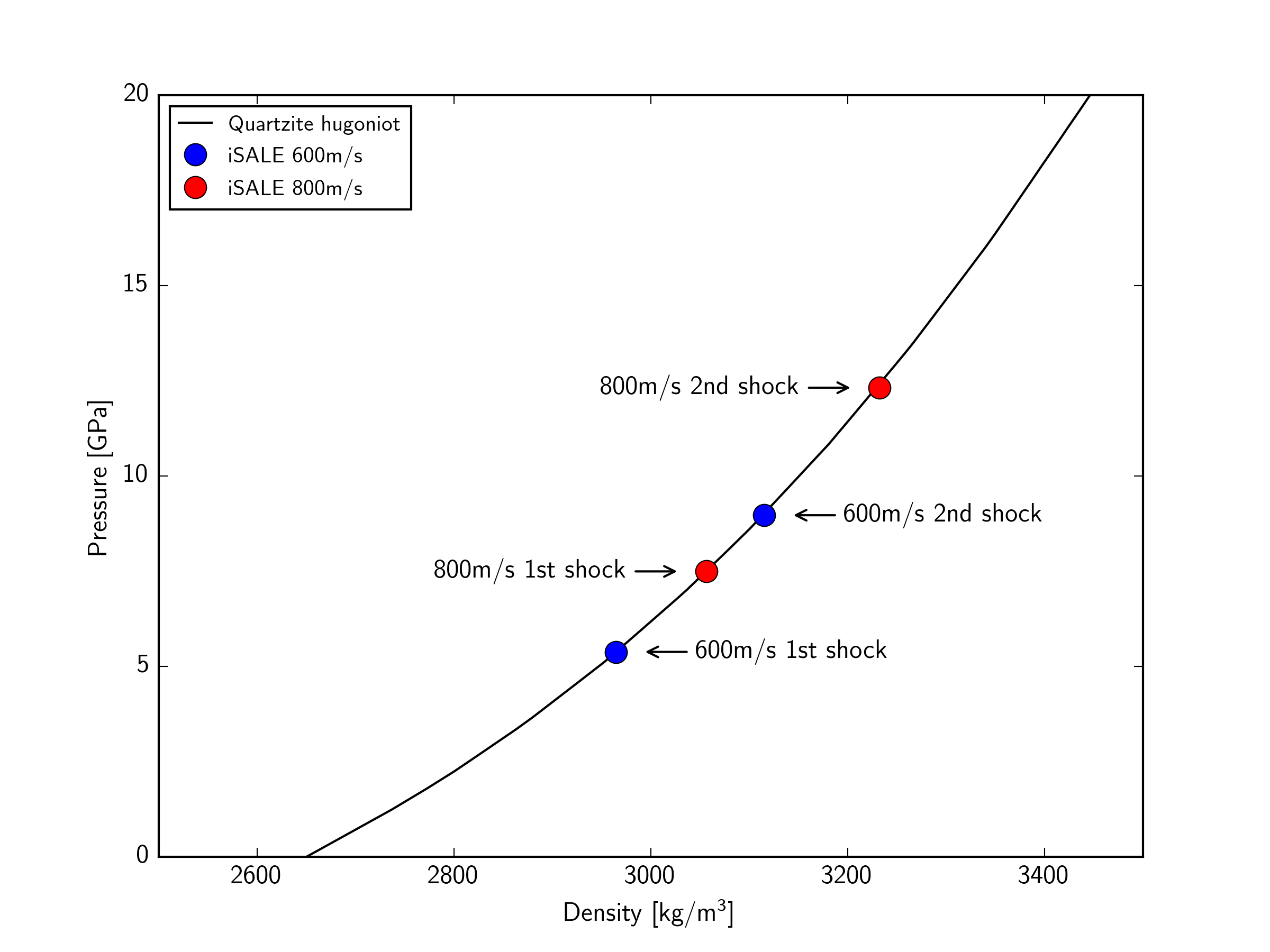
Each of these numerical simulations can be used to compute a point (in fact two, using the shock reflection) on the quartzite Hugoniot. This can be compared with the known Hugoniot curve (which is computed by iSALE at start-up). We can use pySALEPlot to compare the pressure and density in the 1st shockwave and the reflected shockwave with the Hugoniot computed by iSALE.
python Plotting/planar_shock_plot.py
You can view this output in the file: planar_shock_plot.png.
Simulation setup is written in asteroid.inp:
------------------- General Model Info ---------------------------------
VERSION               __DO NOT MODIFY__             : 4.1
DIMENSION             dimension of input file       : 2
PATH                  Data file path                : ./
MODEL                 Modelname                     : Planar-600mps
A cylindrical mesh geometry with a cell size of 0.5 mm and no extension zones:
------------------- Mesh Geometry Parameters ---------------------------
GRIDH                 horizontal cells              : 0           : 100         : 0
GRIDV                 vertical cells                : 0           : 570         : 0
GRIDSPC               grid spacing                  : 5.D-4
CYL                   Cylind. geometry              : 1.0D0
The set-up type is @DEFAULT@ with no gravity field.
------------------- Global setup parameters -----------------------------
S_TYPE                setup type                    : DEFAULT
T_SURF                Surface temp                  : 293.D0
GRAD_TYPE             gradient type                 : NONE
A single impactor object strikes a two layer target. The iron impactor has a @PLATE@ geometry (extending the full width of the mesh) with a half-thickness if 75 cells. The impactor velocity is 0.6 km/s vertically down. In the target, the bottom iron layer extends from cell 1 to cell 200; above this is a quartzite layer, extending from cell 201 to cell 400.
------------------- Projectile ("Object") Parameters --------------------
OBJNUM                number of objects             : 1
OBJRESH               CPPR horizontal               : 75
OBJVEL                object velocity               : -6.D2
OBJMAT                object material               : iron___
OBJTYPE               object type                   : PLATE
------------------- Target Parameters ----------------------------------
LAYNUM                layers number                 : 2
LAYPOS                layer position                : 200         : 400
LAYMAT                layer material                : iron___     : quarzit
The simulation duration is 50 microseconds, with output saved every 0.5 microseconds.
------------------- Time Parameters ------------------------------------
TEND                  end time                      : 5.D-5
DTSAVE                save interval                 : 5.D-7
Deactivate the deviatoric stress model.
------------------- Control parameters (global) ------------------------
STRESS                Consider stress               : 0
Strengthless iron and quartzite material models are used, with ANEOS-derived EoS tables.
-----------------------------------------------------------
MATNAME    Material name          : iron___    : quarzit
EOSNAME    EOS name               : iron___    : quarzit
EOSTYPE    EOS type               : aneos      : aneos
STRMOD     Strength model         : NONE       : NONE
DAMMOD     Damage model           : NONE       : NONE
ACFL       Acoustic fluidisation  : NONE       : NONE
PORMOD     Porosity model         : NONE       : NONE
THSOFT     Thermal softening      : NONE       : NONE
LDWEAK     Low density weakening  : NONE       : NONE
-----------------------------------------------------------
POIS       pois                   : 5.0000D-01 : 5.0000D-01
CHEAT      C_heat                 : 4.4000D+02 : 1.0000D+03
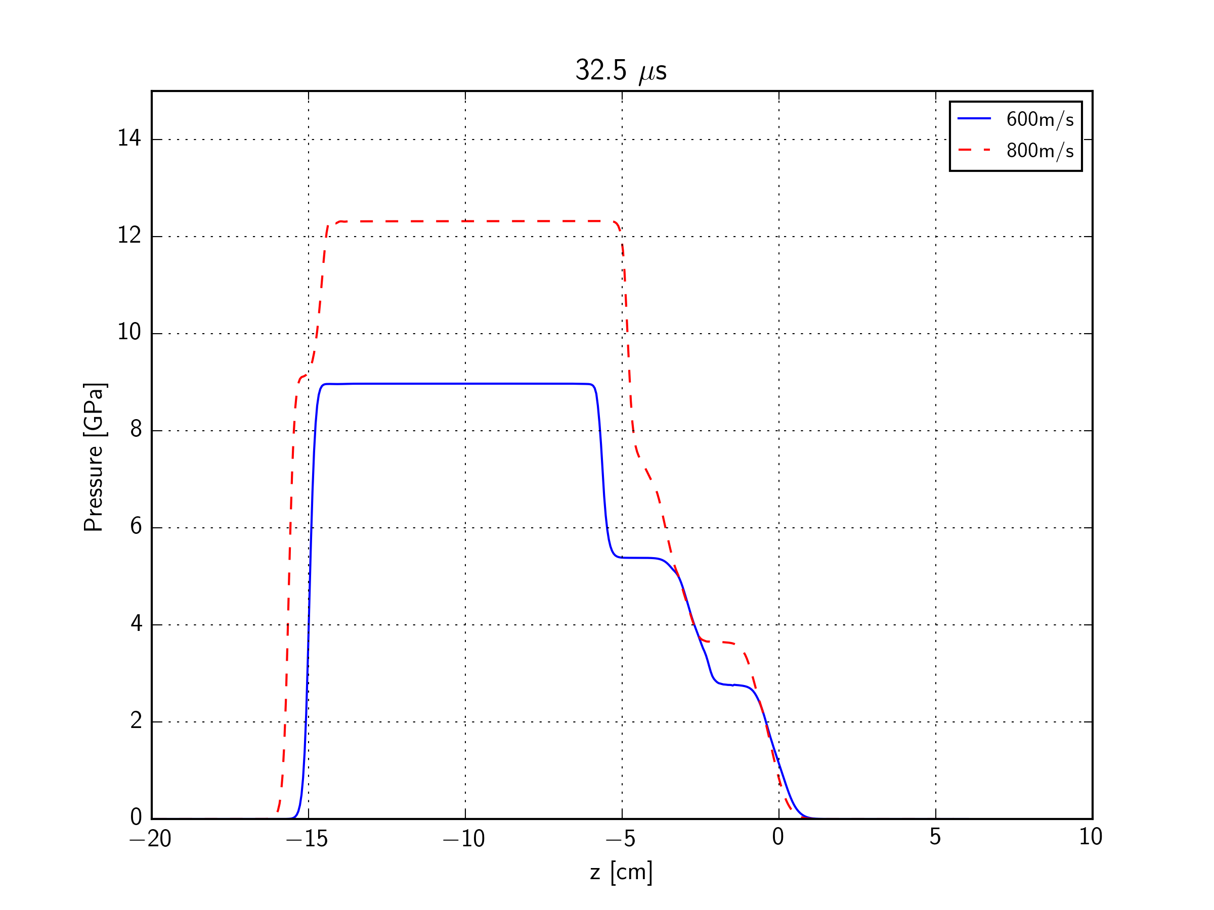
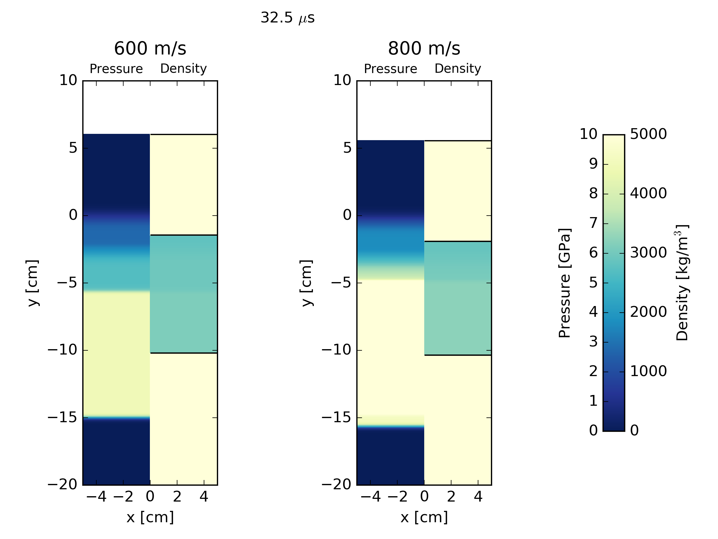
The figures below show the pressure along a vertical profile through the planar impact test at several timesteps: (a) 5 us, (b) 10 us, (c) 15 us, (d) 20 us, (e) 25 us, (f) 32.5 us after the initial impact. Firstly, the shock wave propagates into the target quartzite and the iron impactor. Then, the release wave is initiated at back of impacting plate followed by the reflection of the shock wave into the target and transmitted into the buffer at interface between target and iron buffer plate. At the end, the release wave reaches target. Below the pressure profiles, pressure and density fields are shown at several timesteps.
 |
 |
|---|---|
 |
 |
 |
 |
 |
 |
 |
 |
 |
 |